
Transformer with code Part I - Positional Encoding and Multi-Head Self Attention
Yet another tutorial for Transformer

Previously I posted about the AutoInt model which leverages the self-attention module to model feature interactions. The self-attention module in AutoInt is actually a simplified version. In this post, let’s build the original version in the Transformer paper.1

The Transformer paper is concise and comprehensive. There are many details that lack of discussion. I will try to cover the FAQs one by one in my next few posts.
The Architecture
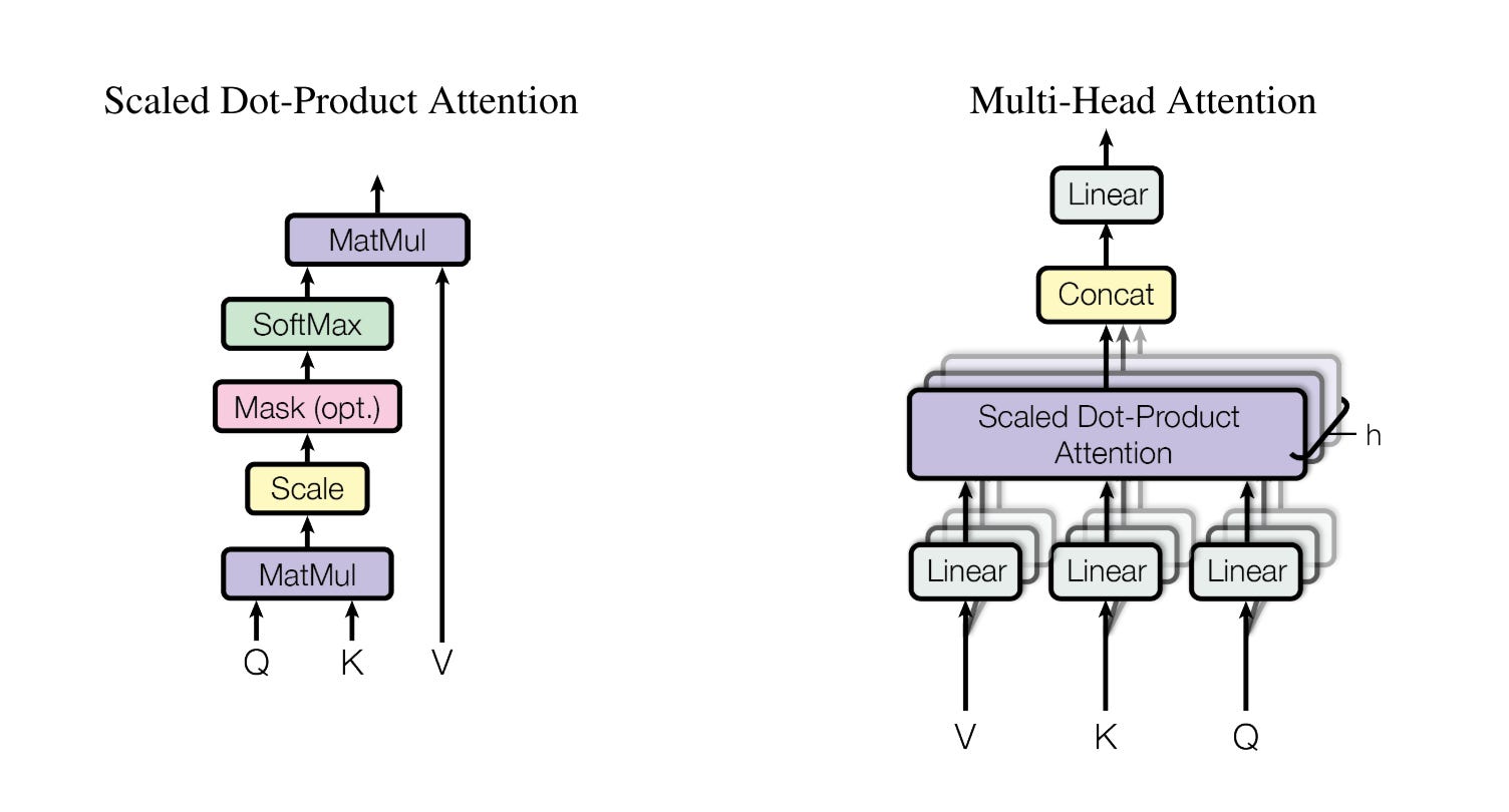
First, let’s have a quick recall of the overall architecture.
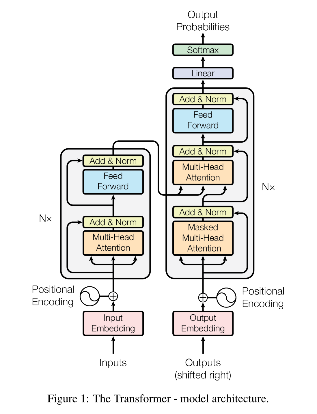
The Transformer consists of 4 major components
On the bottom is the input and output layer. All the input and output tokens are converted to embeddings and element-wise added with an additional positional encoding:
Why do we need positional encoding? That’s because the self-attention module cannot catch the order of the original sequence, so we must inject some information about the relative and absolute position of the tokens in the sequence
On the center-left is a stack of multiple encoders. Here Nx means the depth of the stack. The encoder is composed of
The famous multi-head attention layer, details will be shared later in this post. Notice there are 3 inputs for this layer, they are all the projections of the original input embedding, namely the query, key, and value
Residual and layer normalization layers, the original input is added with the output of multi-head attention and then a layer normalization is applied
A position-wise feed-forward layer, this is just an MLP. After this layer, another residual and layer normalization layer is appended
On the center-right is a stack of multiple decoders. The decoder is composed of:
Two multi-head attention layers
The first one is similar to the attention layer in the encoder but with one major difference. A causal mask must be used to prevent information leaking, the current token in the output sentence can only see the tokens before. More details will be shared later
The second one is often called cross-attention, the major difference is the key and value are from the output of the encoder. And only the query is from the output embedding of the previous self-attention layer
The rest is the same as the residual and normalization layer in the encoder
On the top-right is the final output layer, there is
A linear dense layer that transforms the dimension of output to the vocabulary size. So we can have a prediction logit for every word in the vocabulary
A softmax layer to convert the logits to an actual score
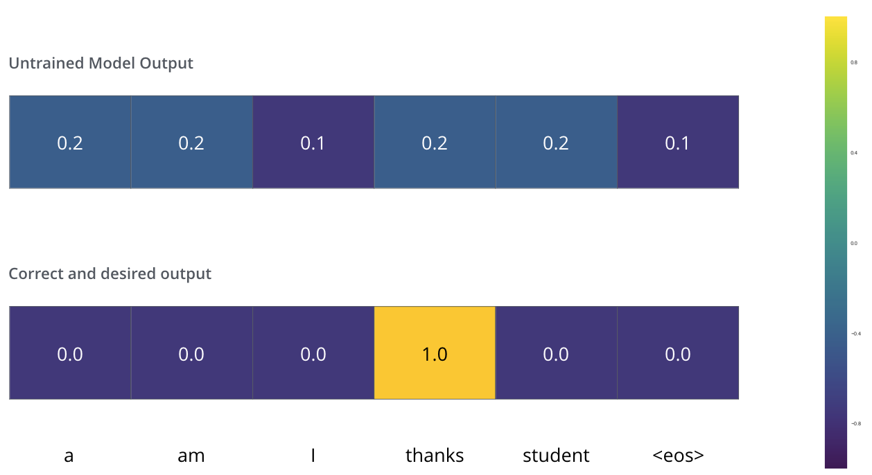
Here is an example from The Illustrated Transformer
In this post, let’s focus on the positional encoding and multi-head attention modules first. They are the most complex and confusing parts.
Positional Encoding
In the paper, the positional encoding is represented as:
Here the range of i is [0, d_model - 1], and d_model is the dimension of the input embedding.
But why? This formula comes from nowhere.
Sine Function
The general ideas come from this post. I translate, summarize and only keep the core ideas.
First, let’s consider other encoding approaches.
Integer encoding is the most straightforward way to encode the positions. But since our length of the sequence is variable. It cannot generalize to unseen or longer sequences and there is no upper bound.
[0, 1] range encoding like min-max scaling. But since the variable length, the interval between two relative positions is also changing. Thinking about one sequence with 4 tokens and another with 5 tokens, the interval between neighbor positions is different, 1/4 vs 1/5. So this approach cannot represent the relative relations well
So our requirements are:
A bounded function that can generalize to any-length sequence
A periodic function that can represent the relative and absolute difference between positions
So cosine and sine functions are both good candidates.
Let’s look at the sine function first, simplify the formula above, and only keep the sine functions. For a position t, the encoding is:
We find that the frequency is negatively correlated with i and the wavelength is positively correlated. This means as the i increases the encoding value will change slower.
This is the same idea as binary encoding but in a reverse order. In the example below, each row represents a binary encoding for numbers in [0, 8]. We can find that as the column index increases, the numbers change faster. So every column in the matrix is encoding different things, and the values won’t be the same.
Why there is a 10000 mysterious number?
That is because the sine function is periodic. If we use a small number like 1, the wavelength will all be small. As position t increases, the encoding values will easily conflict and be close to each other.
Cosine Function
So why there is another cosine? It turns out that using cosine at odd positions allows the model to learn the relations of relative position.
With the cosine function, for any fixed offset k, PE_pos+k can be represented as a linear function of PE_pos:
This linear function can be easily constructed using sine and cosine functions.
The Code
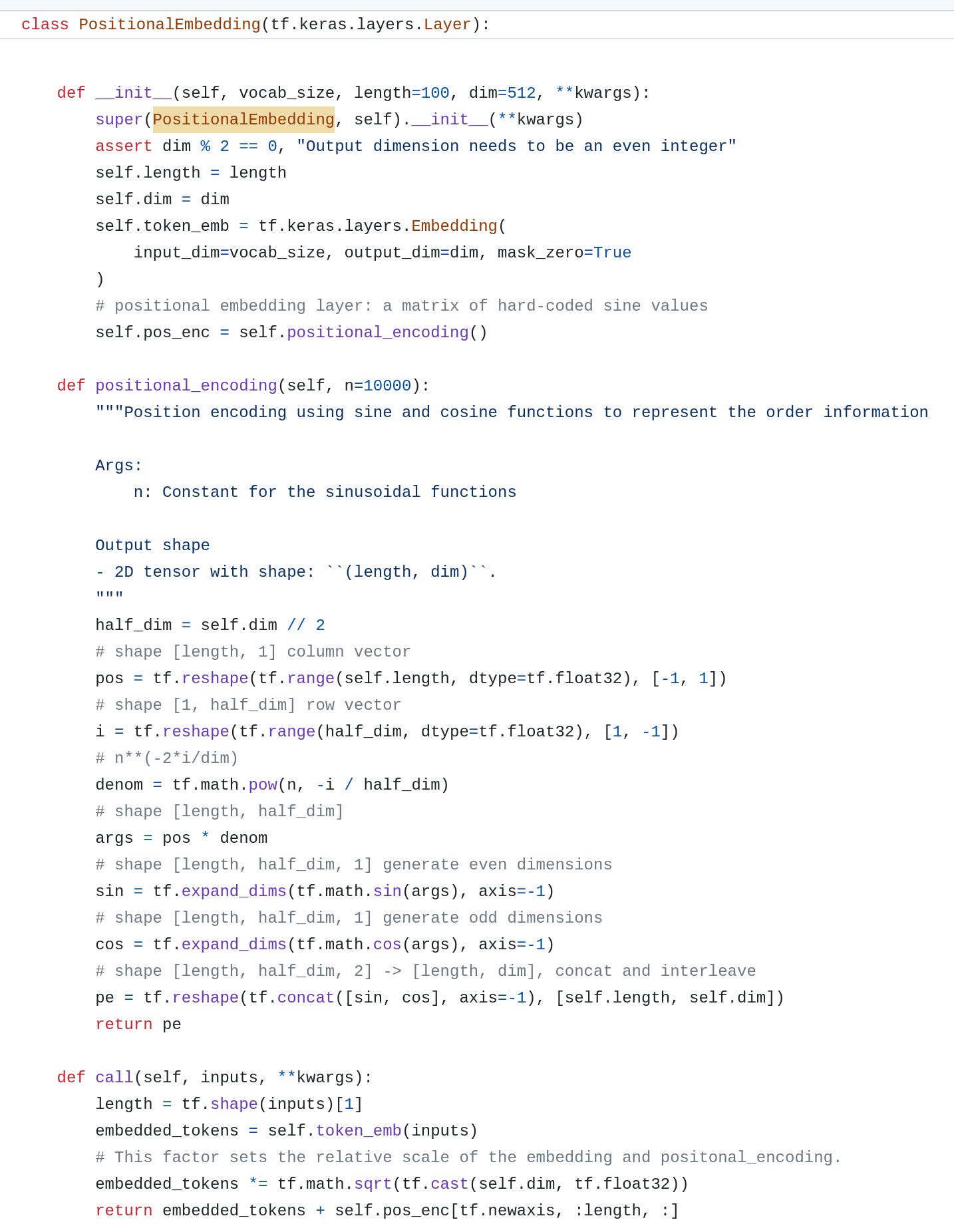
I refer to the implementation in the machinelearningmastery and use TensorFlow to rewrite it. The source code is here.
Notice here I use tf.concat and tf.reshape functions to interleave the values from sine and cosine functions. length is the sequence length and dim is the dimension of token embedding.
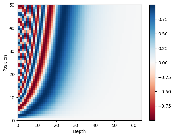
Let’s plot the sine and cosine values separately. We can see the trend is similar, as the depth increase, the values change slower.
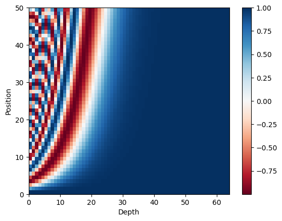
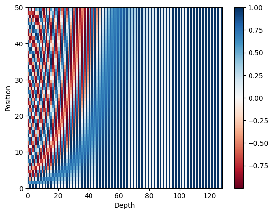
Put them together, we can see interleaved waves.
There is also an interesting feature regarding the dot product of two positional encodings:
The result of the dot product only depends on the distance k
The distance is unidirectional, i.e. the dot product is symmetric
Pick the middle position 24 and plot the dot product. We can see the values are symmetric.
Multi-Head Attention
The main ideas are already covered in my AutoInt post. Here I only highlight the difference and share this complete version of the code.
In Transformer, the input Q, K, and V are different in the cross-attention layer between the encoder and decoder, just like I mentioned before. But in AutoInt, the Q, K, and V are all the same, from the input features
Why do we need to scale the weights before the softmax? That’s for speedup the training process. Since the sequence can be long, the output of Q multiplied by K can be huge. If we directly feed this to softmax, it can be saturated and the gradient can be small
Why multi-head? This is just for increasing the capacity of the model and empowering it to catch different attention patterns across multiple heads
There is no masking in the AutoInt because there is no padding in the input features. But in Transformer, the input length is variable. So the padding zeros must be masked. And furthermore, another causal masked must be used for the output sequence
The Code
TensorFlow already has an official implementation. But it contains too many redundant codes, so I simplify it and only keep the key parts for easy understanding.
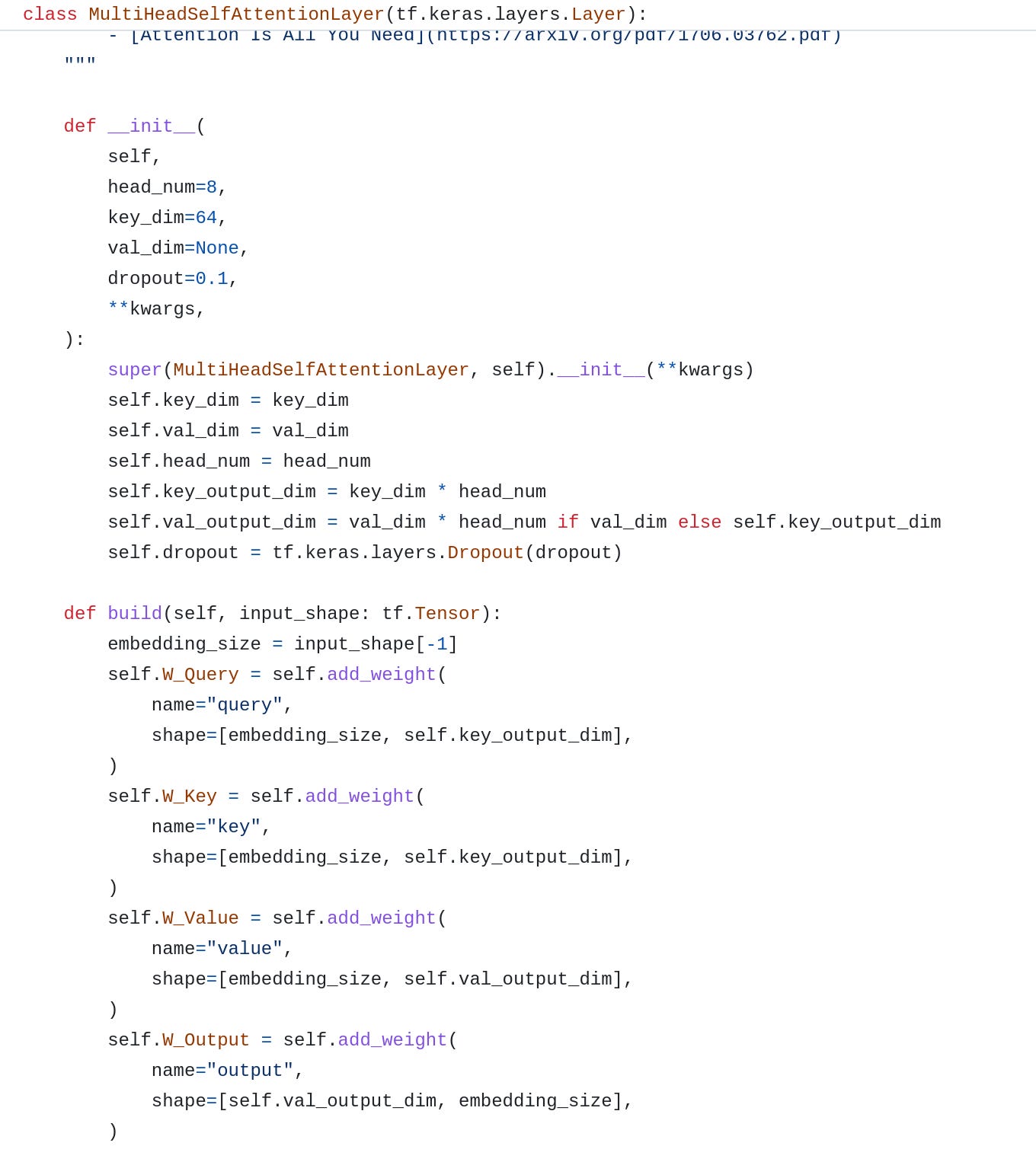
Here is the code.
Initialize the Q, K and V weight matrices. And an extra output projection matrix.
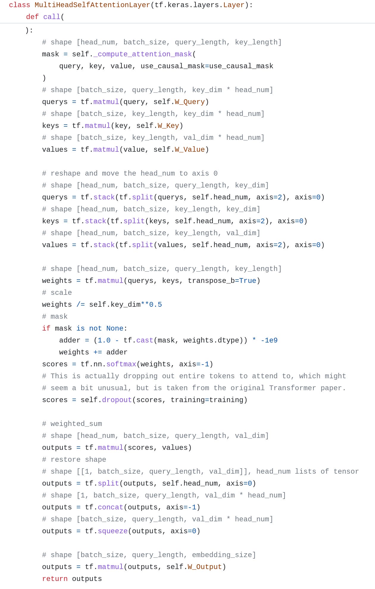
In the main call function, most parts are the same as the implementation in AutoInt, but the inputs are three items Q, K, and V instead of one single input:
Notice the embedding dimensions of the query and key must be the same, this is the requirement for weight calculation
The sequence_length of the key and value must be the same, this is the requirement for value aggregation
Masking is implemented by adding a very big negative number -1e9. After processing by Softmax, the logit will be close to zero and be ignored
There is an extra dropout layer that I cannot find in the original paper, I just followed the official implementation from TensorFlow
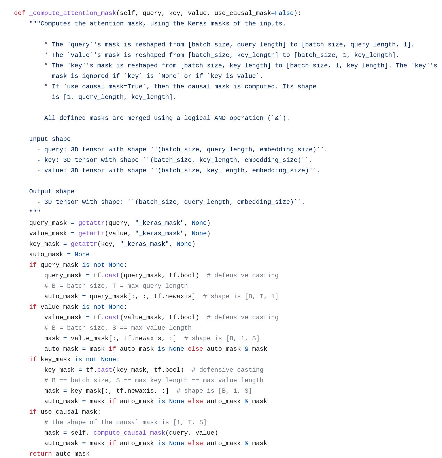
Computing the mask, this part is almost the same as the TensorFlow implementation. Notice that we need to consider the mask from Q, K, V, and union them together.
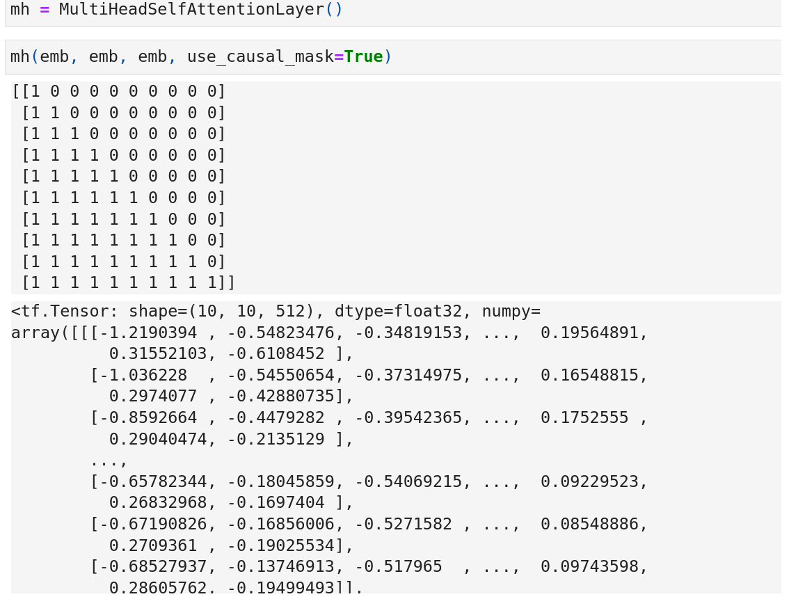
The last part is computing the causal mask. This is actually a lower triangular matrix.
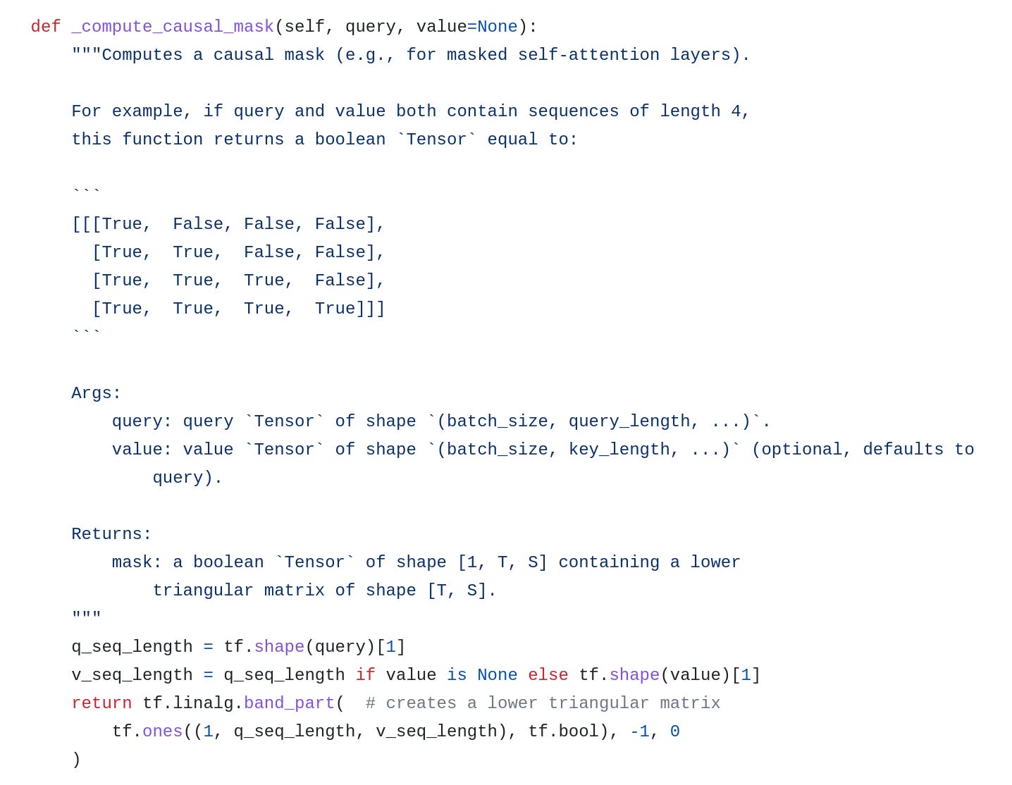
Why a lower triangular matrix? Imagine our output sequence is “I love cats”. The corresponding causal mask will be:
Here row 0 represents the mask from I to the other 3 words including itself. And it’s the same for other rows. So for the word I, it only considers I itself. For love, it considers both I and love. For the word cats, it considers all the 3 words.
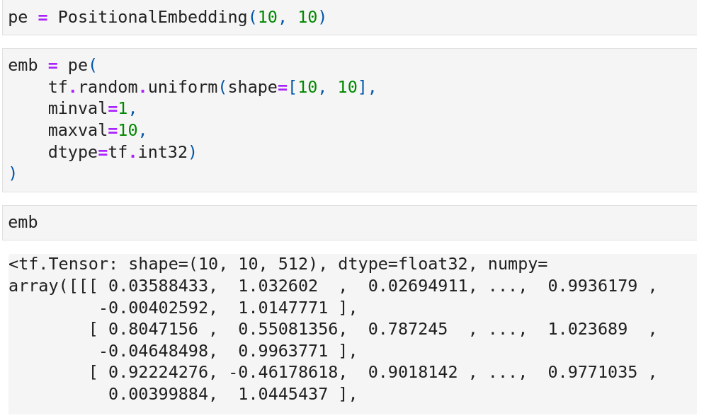
Run a random example and print the mask, we can see the causal mask is as we expected.
Input and Output
Another confusing thing is the input and output for the Transformer model.
For the training phase, the sample is like:
encoder_input: i have more than enough.
decoder_input: [start] j'en ai plus que marre . [end]
target: j'en ai plus que marre . [end]
Two sentinels [start] and [end] are added as special tokens, so the target can keep the first-word j'en for training and the model will also know when to end.
And since there is causal masking, all the logits for the 5 output words are calculated in parallel and there are 5 true labels in one sample.
For the inference or testing phase, the sample is like:
encoder_input: i have more than enough.
decoder_input: [start] → decoder_ouput: j'en
decoder_input: [start] j'en → decoder_ouput: ai
…
decoder_input: [start] j'en ai plus que marre . → decoder_ouput: [end]
Notice the output is generated one by one or multiple by multiple using beam-search because we don’t know the target beforehand. This is why there is a shifted right mark below the outputs of the Transformer architecture picture.
That’s all for today. It’s a super busy week, so I will skip the weekly digest for this week :).
https://arxiv.org/pdf/1706.03762.pdf
dropout is mentioned on Page 8(https://arxiv.org/pdf/1706.03762.pdf):
Residual Dropout We apply dropout [33] to the output of each sub-layer, before it is added to the
sub-layer input and normalized. In addition, we apply dropout to the sums of the embeddings and the
positional encodings in both the encoder and decoder stacks. For the base model, we use a rate of
Pdrop = 0.1.
thanks for this great post! detailed explanation.
I have two questions for positional embedding:
1. why `assert length % 2 == 0` is required? why can't the sequence length be odd number?
2. `denom = tf.math.pow(n, -i / half_dim)` should be `denom = 1 / tf.math.pow(n, -i / half_dim)`, right?