

Deep & Cross Network for Ad Click Predictions
Deep & Cross Network for Ad Click Predictions
Explicitly catch high-order feature interactions

In this post, let’s continue our journey - revisiting the first version of Deep&Cross Network (DCN) from Google1.
It follows the ideas from the W&D model and upgrades the wide part to a Cross Network
Compared to W&D which needs manual feature engineering work, the Cross Network part from DCN can explicitly model high-order feature interactions and the order can be controlled by layer depth
The extra time complexity brings by Cross Network is limited and linear which makes the model fast to train
There is a flaw in the feature cross method. DCN can only model a special format of feature interaction, so there are DCN V2 and xDeepFM in the next that mitigate this issue
Paper reading
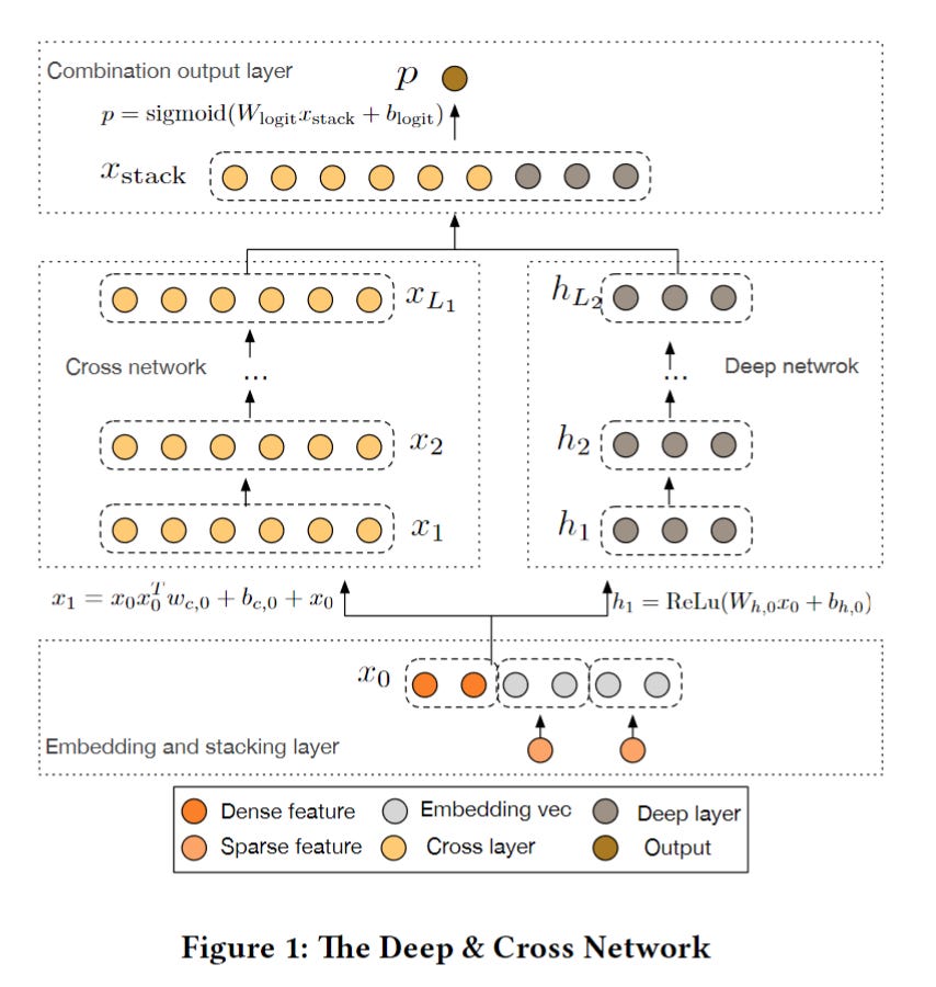
The Structure
First, let’s take a look at the whole structure of DCN:
The dense features are directly fed into the network. The sparse features are converted to embeddings and concatenated with dense features. This is a common approach nowadays
Same as the W&D model, it has a DNN part on the right which consists of multiple MLP layers using the activation function Relu
On the left, the wide linear part is replaced by a stack of feature interaction layers call Cross Network
In each layer, the Cross Network introduces a higher-order of feature interactions by bit-wise embedding multiplication
The dimension is always the same throughout all the layers
The output of Cross Network and Deep network are concatenated and transformed by a linear model to a logits
Cross Network
The Cross Network is the core of DCN, let’s see how it works.
Cross Layer
The Cross Network consists of multiple cross layers. The output of each cross layer is made from 3 parts
A feature crossing part, X0 is the original input feature, X' is the transpose of the input X of the current layer, and W is the weight parameters. Then the 3 parameters are matrix-multiplied together
A bias parameters have the same dimension as X0 and X
The input of the current layer X, which has the same dimension as X0

The math formula shows the same idea but clearer:
l means the l-th cross layer
W and b are the learnable weights and bias
X is the embedding input/output for each layer
How to explicitly model any-order feature interaction?
The proof in the paper is super trivial. Let’s take a concrete example for easy understanding.2
For simplicity, suppose the input X0 is:
And there is no bias term, then
We can see from the red-marked Xs, this contains all the polynomial combinations of features.
What’s the problem with this formula?
It looks perfect at first sight. But the representation ability is limited. We can understand this in two ways:
The weight for different feature cross terms are the same, this doesn’t make sense. Let’s focus on the weights this time, we can see the weights in each column are forced to be the same
\( X_1 = \begin{bmatrix} {\color{red}w_{0, 1}}x_{0,1}^2+ {\color{red}w_{0,2}}x_{0,1}x_{0,2}+ x_{0, 1}\\ {\color{red}w_{0, 1}}x_{0, 2}x_{0,1}+ {\color{red}w_{0,2}}x_{0,2}^2+ x_{0, 2} \end{bmatrix}\)Actually, the second matrix multiplication of feature crossing in the formula is a scalar. This makes the output of feature interaction a scalar multiple X0 (Please notice that the scalar comes from X0, so it still involves polynomial combinations). So the final output is limited to a special form
\(\begin{align*} X_1 &= X_0X_0^TW_0 + X_0 \\ &= \begin{bmatrix} x_{0,1} \\ x_{0, 2} \end{bmatrix} \begin{bmatrix} x_{0,1} x_{0, 2} \end{bmatrix} \begin{bmatrix} w_{0,1} \\ w_{0, 2} \end{bmatrix} + \begin{bmatrix} x_{0,1} \\ x_{0, 2} \end{bmatrix} \\ &= \begin{bmatrix} x_{0,1} \\ x_{0, 2} \end{bmatrix} (x_{0,1} w_{0,1} + x_{0, 2}w_{0,2}) + \begin{bmatrix} x_{0,1} \\ x_{0, 2} \end{bmatrix} \\ &= \begin{bmatrix} x_{0,1} \\ x_{0, 2} \end{bmatrix} ( x_{0,1} w_{0,1} + x_{0, 2}w_{0,2} + 1 ) \\ &= \begin{bmatrix} x_{0,1} \\ x_{0, 2} \end{bmatrix} ( {\color{red}scalar + 1} ) \end{align*}\)
Time Complexity
The good thing about Cross Network is for each layer it only brings a d-dimension weight and another d-dimension bias. So the total time complexity is linear to the depth of layers. This is much smaller than the time complexity of DNN layers.
Show me the code
The Cross Network:
Build weights and biases according to the input embedding dimension size. Note that we must provide a name for these customized weights, or we will encounter an error when saving the model (Messy TensorFlow 😒)
Then calculate the output for each cross layer. Note that it’s much better to calculate the second part X'*W first in terms of memory and computation complexity
Another tricky thing is we must specify the axis when squeezing because the embedding_size is dynamic (None while running) and TensorFlow doesn’t know whether it should be squeezed or not

The rest part is easy, just concatenate the output with DNN then add another dense layer.

Weekly Digest
MLOps Landscape in 2023: Top Tools and Platforms. An overview of popular ML tools
LLM based Chatbots to query your Private Knowledge Base. Love this article, imagine that we can also take the recommendation candidates as our Knowledge Base and use LLM to do the ranking
The Problem with Timeseries Data in Machine Learning Feature Systems. Good practice on using Timestamps. In one word, always use a long unix timestamp, no complex data structures
Choosing Sequential Testing Framework — Comparisons and Discussions. How to mitigate the peeking issue while ab testing?

https://arxiv.org/pdf/1708.05123.pdf
https://zhuanlan.zhihu.com/p/347659531