

Deep Learning Recommendation Model for Personalization and Recommendation Systems
Deep Learning Recommendation Model for Personalization and Recommendation Systems
Best practice for recommendation systems from Facebook

In this post, let’s look at Facebook’s recommendation system. This paper is quite different from our previous shared papers. In this paper, the modeling work is only a small part, and half of the content is about the training infrastructure. It shows us a big picture of an industrial recommendation system.
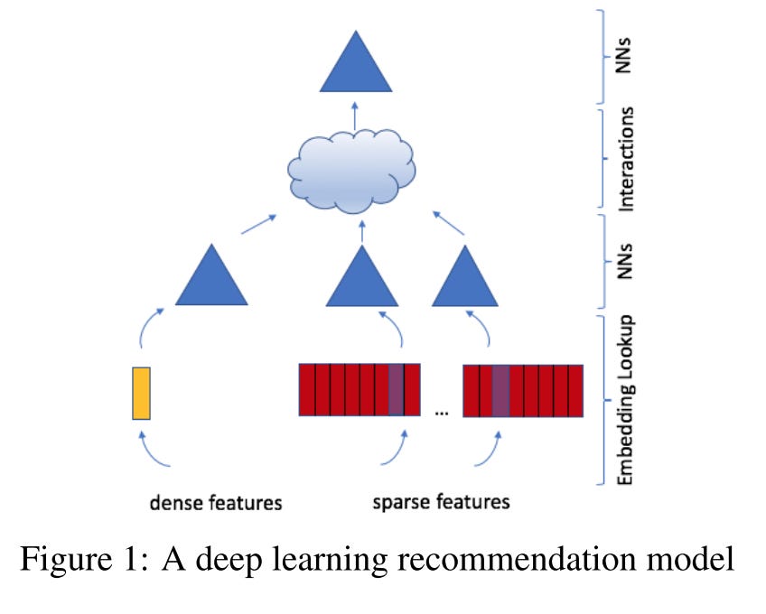
The Deep Learning Recommendation Model (DLRM)1 consists of 4 components:
Bottom fully-connected (MLP) layers transform the dense input features
Embedding tables retrieve embeddings for sparse features
A dot production interaction layer to perform feature interactions on sparse embeddings from component 2 and transformed dense embeddings from component 1
Top MLP layers to extract the final prediction from the dense features and feature interactions
Real-world large-scale recommendation systems require large and complex models to capitalize on vast amounts of data. DLRM utilizes model parallelism on the embedding tables to mitigate memory constraints while exploiting data parallelism to scale out compute from the fully-connected layers
Overall Architecture
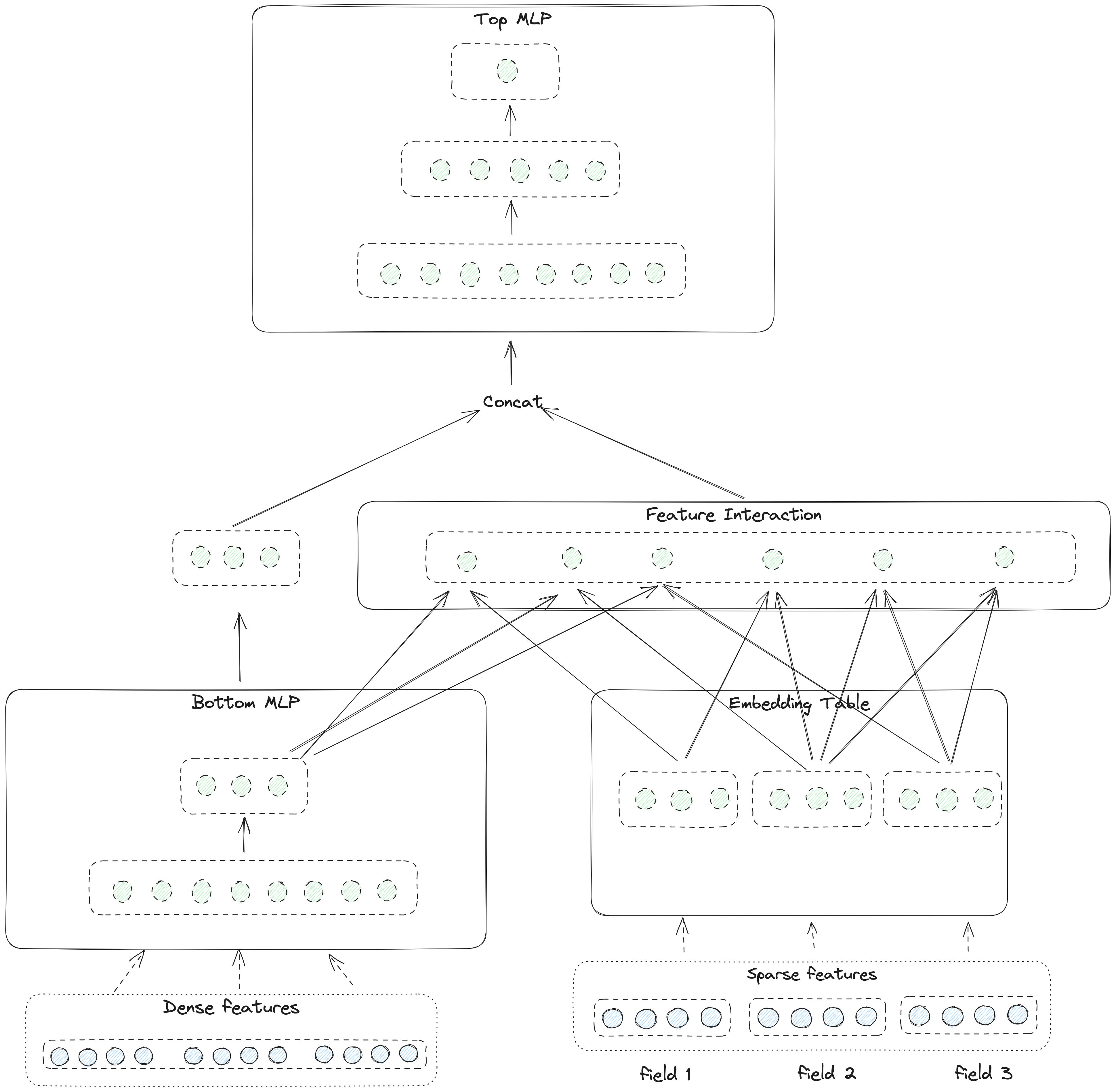
The architecture diagram above is sketchy (Maybe this is also Facebook-style 😄, papers from other companies always give a detailed architecture diagram). Let me share a clearer picture here.
On the bottom left are all the dense features. On the bottom right are all the sparse features
For dense features, they are fed into multiple MLP layers here called bottom MLP for dimension reduction and implicit feature interaction. Notice that the output dimension of the bottom MLP is the same as the embedding dimension of a single sparse feature. This is the precondition of interaction between dense and sparse features
For the sparse features, embeddings are retrieved from embedding tables
A dot product feature interaction is applied to:
all the dense and sparse feature embeddings
for instance, suppose in the picture we have 1 dense embedding and 3 sparse embeddings, the final output size will be 4 * 3 / 2 = 6
Then the original dense embedding will be concatenated with the output vectors of the feature interaction layer and fed into another multiple MLPs called the Top MLP layers
The last layer of the Top MLP output the prediction
Here DLRM only models the second-order feature interaction. Recall that other models like xDeepFM and AutoInt, they all support any-order feature interactions and prove that are useful.
In this paper, the Facebook team makes a trade-off between model performance and training cost. They prefer cost reduction.
We argue that higher-order interactions beyond second-order found in other networks may not necessarily be worth the additional computational/memory cost.
Implement the Feature Interaction
TensorFlow Recommender library already provides the implementation of the feature interaction component. Their implement is clean and pretty, I won’t bother to re-create the wheel here. Let’s go through the code here.
First, the input is a list of batched feature embeddings, like [[batch_size, feature_dim]]. Then the input will be transformed into a shape [batch_size, num_features, feature_dim] and the embedding matrix will be multiplied by itself to get all the feature interaction pairs. Recall that here each value of the output matrix is actually a dot product result.

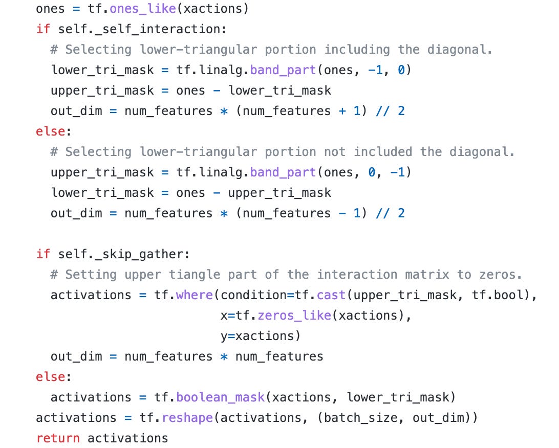
Remember that the matrix is symmetric but actually we only need the upper or lower half of the result. So another mask operation is applied. Here they use a special function called tf.linalg.band_part in TensorFlow, we can easily get the upper or lower triangular part, as listed below.
 tf.linalg.band_part(input, 0, -1) ==> Upper triangular part.
 tf.linalg.band_part(input, -1, 0) ==> Lower triangular part.
 tf.linalg.band_part(input, 0, 0) ==> Diagonal.
After masking, all the output will be flattened and transformed to shape [batch_size, out_dim]. Here we can choose either to include the self-interaction (the diagonal) or not.
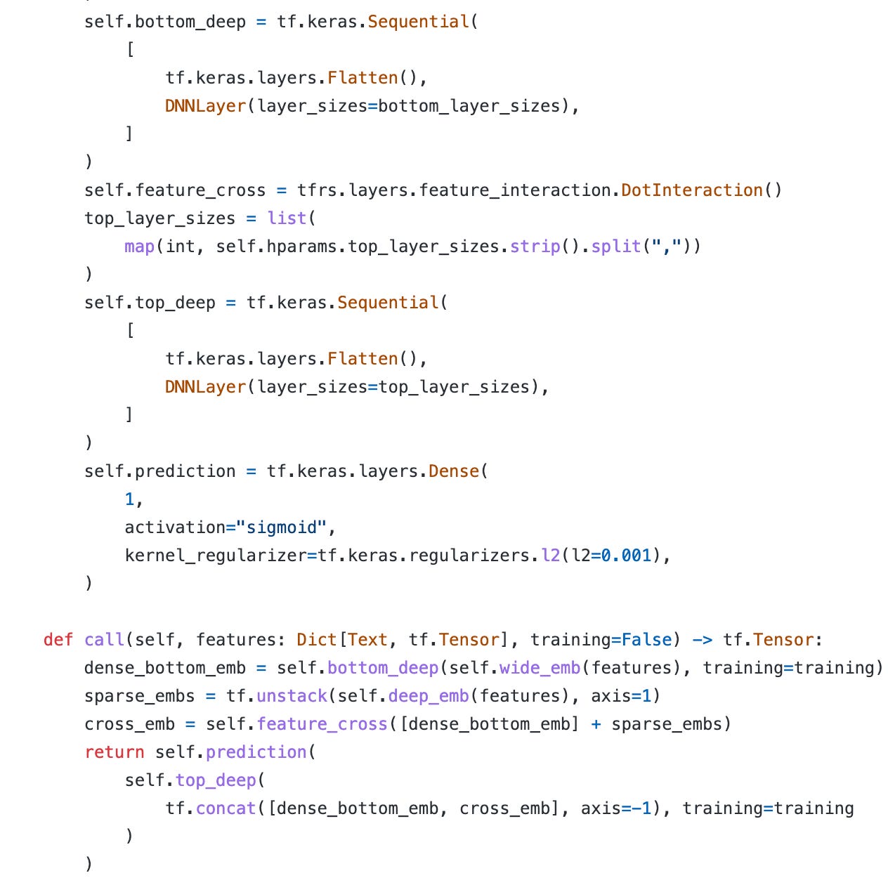
Then the final work is just defining all the embedding and MLP layers and concatenating them as the architecture shared above.
Since DLRM requires dense feature input, but MovieLens-1M dataset doesn’t have dense features. I spent some time preparing the Criteo dataset which is also the experiment dataset for the DLRM paper. I haven’t finished running the experiment yet ( the data is huge). I will benchmark all the models I shared before and give the result later.
Parallelism
The other part of the paper is all about parallel training and optimizing the training speed.
DLRMs particularly contain a very large number of parameters, up to multiple orders of magnitude. Hence, it is important to parallelize these models efficiently in order to solve these problems at practical scales.
Let’s take a close look at the architecture from memory and computation perspectives.
In industry, there are huge amounts of sparse features and the embedding tables will also be huge. So for the bottom embedding table, it requires big memory capacity for storage and high memory bandwidth for embedding lookup
For the feature interaction layer, it requires fast communication to get all the embeddings for interaction calculation
For the top MLP layers, it’s purely compute-dominated and requires fast computation resources

Model Parallel and Data Parallel
Therefore, model parallelism is preferred for embedding tables to mitigate the memory bottleneck produced by the embeddings. Data parallelism is preferred for MLPs since this enables concurrent processing of the samples on different devices and only requires communication when accumulating updates.
DLRM uses a combination of model parallelism for the embeddings and data parallelism for the MLPs.
A butterfly shuffle operation is required for communication between embedding tables and MLPs. But PyTorch and Caffe2 don’t support this operation, so the author implements the operation by explicitly mapping the embedding operations to different devices. They shared the code in Github.

Experiments
In the paper, they use random and synthetic datasets for training speed verification. In order to keep the original distribution and also consider data privacy, they create a complex algorithm to generate the synthetic data. It’s quite trivial and hard to understand, I will skip this part here.
And they use the Criteo dataset for model performance comparison. They also emphasize that this is without extensive tuning of model hyperparameters.
They use the DCN as the baseline. (🤔Why not use xDeepFM which is stronger than DCN?) We can see the performance is consistently better.

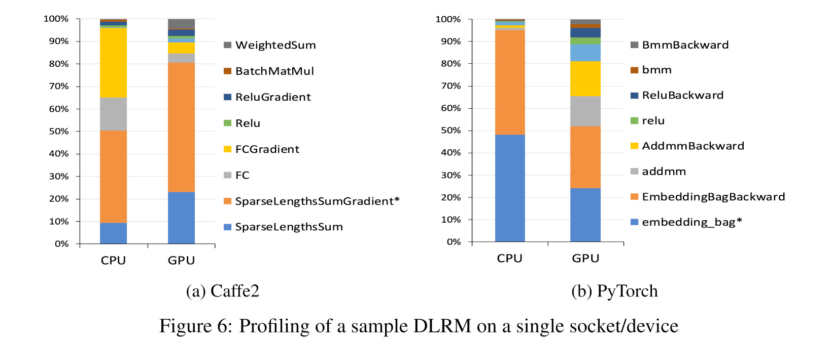
They also profiled the training performance on random and synthetic datasets. The majority of time is spent performing embedding lookups and fully connected layers. On the CPU, fully connected layers take a significant portion of the computation, while on the GPU they are almost negligible.
Weekly Digest
This week, I will only share one special article. It’s super long but contains many impressive insights.

How to do great work from Paul Graham
Some highlights:
The first step is to decide what to work on. The work you choose needs to have three qualities: it has to be something you have a natural aptitude for, that you have a deep interest in, and that offers scope to do great work.
Four steps: choose a field, learn enough to get to the frontier, notice gaps, explore promising ones. This is how practically everyone who's done great work has done it, from painters to physicists.
One sign that you're suited for some kind of work is when you like even the parts that other people find tedious or frightening.
The following words precisely describe the progress of writing a blog 🎯.
The reason we're surprised is that we underestimate the cumulative effect of work. Writing a page a day doesn't sound like much, but if you do it every day you'll write a book a year. That's the key: consistency. People who do great things don't get a lot done every day. They get something done, rather than nothing.
If you do work that compounds, you'll get exponential growth. Most people who do this do it unconsciously, but it's worth stopping to think about. Learning, for example, is an instance of this phenomenon: the more you learn about something, the easier it is to learn more. Growing an audience is another: the more fans you have, the more new fans they'll bring you.
The trouble with exponential growth is that the curve feels flat in the beginning. It isn't; it's still a wonderful exponential curve.
I’m still reading it, let’s read together!
https://arxiv.org/pdf/1906.00091.pdf