

From FM to DeepFM, the almighty Factorization Machines
From FM to DeepFM, the almighty Factorization Machines
Build a FM ranker, candidate retriever and DeepFM ranker using TensorFlow

In this post, let’s revisit the classic ranking algorithm Factorization Machines and the successor DeepFM in the Deep Learning era.
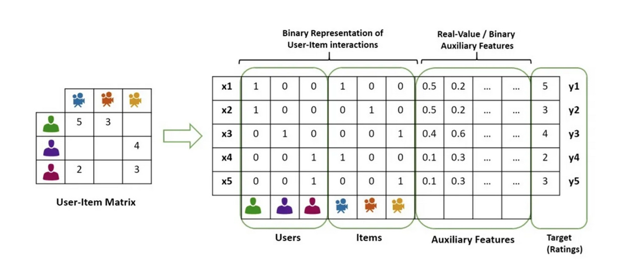
The idea of Factorization Machines (FMs from now on) is to learn a polynomial kernel by representing high-order terms as a low-dimensional inner product of latent factor vectors. In other words, learning feature interactions using similarity of embeddings1
FM is very efficient at learning second-order feature interactions. And besides ranking, it can also be transformed into a Candidate Retriever (CR from now on) which makes it still useful in the Deep Learning dominated recommender system today
The DeepFM is an end-to-end model that combines the power of FM for recommendation and deep learning for feature learning in a new neural network architecture to learn both low and high-order feature interactions2
DeepFM has a shared input to its “wide” and “deep” parts, with no need for feature engineering besides raw features which makes it effortless compared to the W&D model
These two algorithms are super popular in the recommender system and let’s follow our tradition, ignore trivial details in the paper and focus on the main ideas.
FM
Core Concept
Recall the linear regression model, here y is the target, w0 is the bias, wi is the i-th weights, xi is the i-th feature value.
The biggest disadvantage of the model is, if we want to capture the 2nd order feature interaction, like a job SDE and a location in San Francisco, we have to do this manually. Adding a weight like:
This is a pretty heavy workload. FM solves it by introducing a generalized order 2 polynomial.
And the weight of the 2nd order feature can be calculated by the dot product of 2 vectors, suppose the length of each vector is k.
Recall the idea of the Matrix Factorization (MF) model, actually the FM shares the same idea. The only difference is the features are not limited to the user and item IDs.3
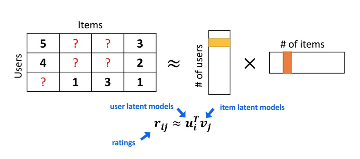
In FM, we will learn latent vector pairs for each user and item interaction feature.
So we can say that:
FM is a generalization of MF and MF is a special case of FM
Optimize the Time Complexity
The original formula basically means the time complexity of the FM model is O(k*n^2). This is quite slow in terms of trillions of features used in industry.
But fortunately, it can be optimized to an O(k*n) complexity, here the deduction is:
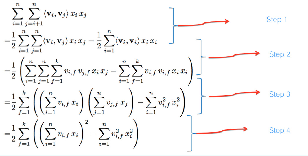
I won’t go through too many math details here, you can refer to this post for the detailed explanation.
This transformation is critical, all of our implementation will be based on it.
Implementation
There are many implementations for FM, you can find some examples from Microsoft. Here I prefer to use TensorFlow and don’t want to involve other tech stacks.
A naive example is like this one, which uses the native TensorFlow APIs without any high-level Keras layers.
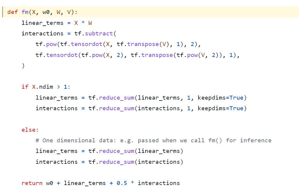
We can see here the calculation here follows exactly the math formula. After getting the interaction value, then added it to the linear and bias value.
Also, let’s look at another example from DeepCTR which is implemented in TensorFlow 1.0.
Here the feature vector X disappears, why?
Embedding can be considered as a one hot feature vector X multiply an embedding table matrix V
In the DeepCTR’s version, the inputs are already the outcome of the multiplication of X and V. So these 2 versions are actually equivalent
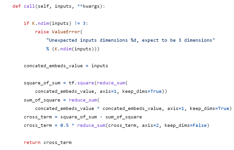
Combine these 2 versions together, and let’s re-implement it in TensorFlow 2 and remove redundant code.

And define a ranking model using this FM layer. Here I separate linear user and item features from each other intentionally. I will explain more about this later.
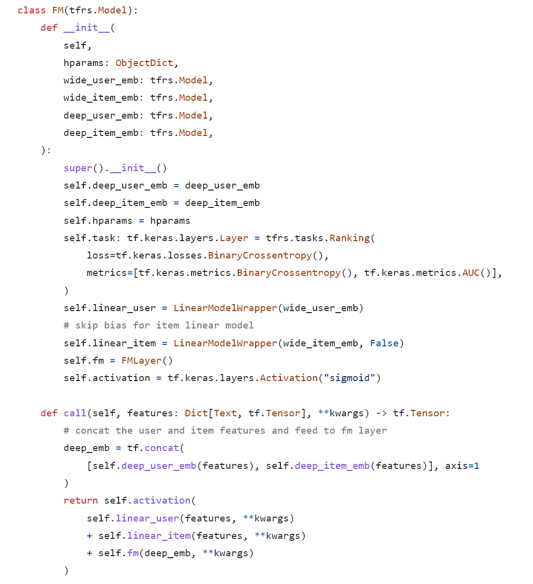
That’s it. The final logits = sigmoid(bias + linear + fm).
FM as a CR
Deep ranking models dominate the recommender ranking system nowadays and they outperform FM a lot on ranking metrics. Is FM still useful?
Yes, it can be easily transformed into a CR.
Compared to collaborative filtering based CR or two-tower based CR, FM has a clear advantage in explicit modeling feature interactions.
Split the Features
Suppose we have in total n features and m user features, then the features can be split into a user feature part Vu and an item feature part Vk: 4
The original FM formula is equivalent to (ignore the x features for simplicity):
This means the target is equal to the following:
y = bias + linear_user_part_score + linear_item_part_score + user2user_interaction_score + item2item_interaction_score + user2item_interaction_score
Because in the online recall scenario, the querying user is the same. So for each item, the user part is the same. So we only need to calculate the item part score:
user_item_matching_score = linear_item_part_score + item2item_interaction_score + user2item_interaction_score
And notice that:
Simplify the above formulas:
user_item_matching_score = item_part_score + dot<sum_of_user_vector, sum_of_item_vector>
So we can build the user and item embedding as:
Then the dot product of these 2 embeddings will be our target matching score.
Implementation
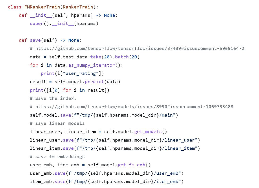
In the training phase, we need to separate the user and item features and save the corresponding models as:
When generating embeddings, we just follow the math calculation:
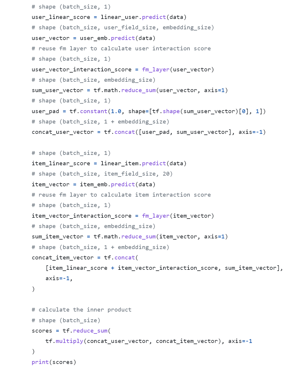
And let’s add the user part score to verify the correctness.
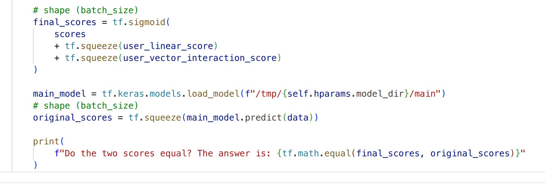

That’s it. Then we can save all the item embeddings to any ANN search engine like Faiss and deploy the index to the online service.
DeepFM
We already fully understand the theory of FM, then DeepFM is just easy peasy!
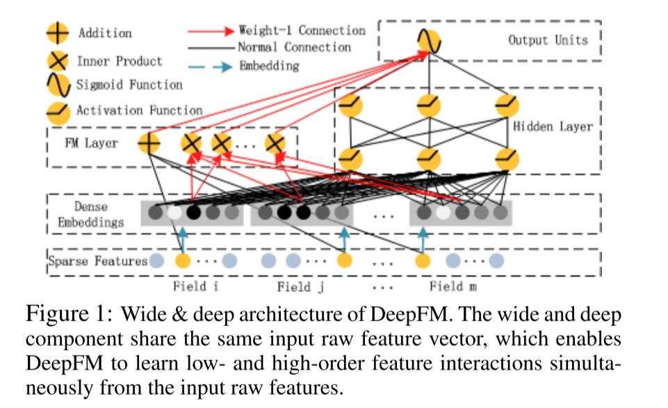
As we can see in the picture, the prediction logits of DeepFM is:
y = sigmoid(linear_score + fm_score + dense_score)
Notice that there are 2 unique requirements:
The embedding dimension of all features are the same, to support dot product for FM
The embeddings are shared between the FM and Dense part
Implementation
Sharing a similar structure with the W&D model, the forward pass of DeepFM is:
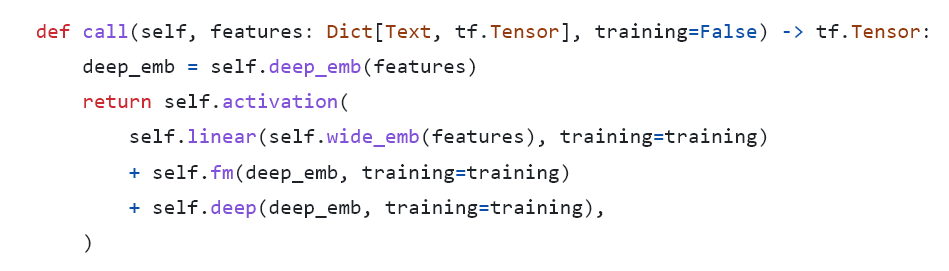
FM layer is just the same code as I shared before. Notice the deep_emb is shared between FM and Deep layers.
Example
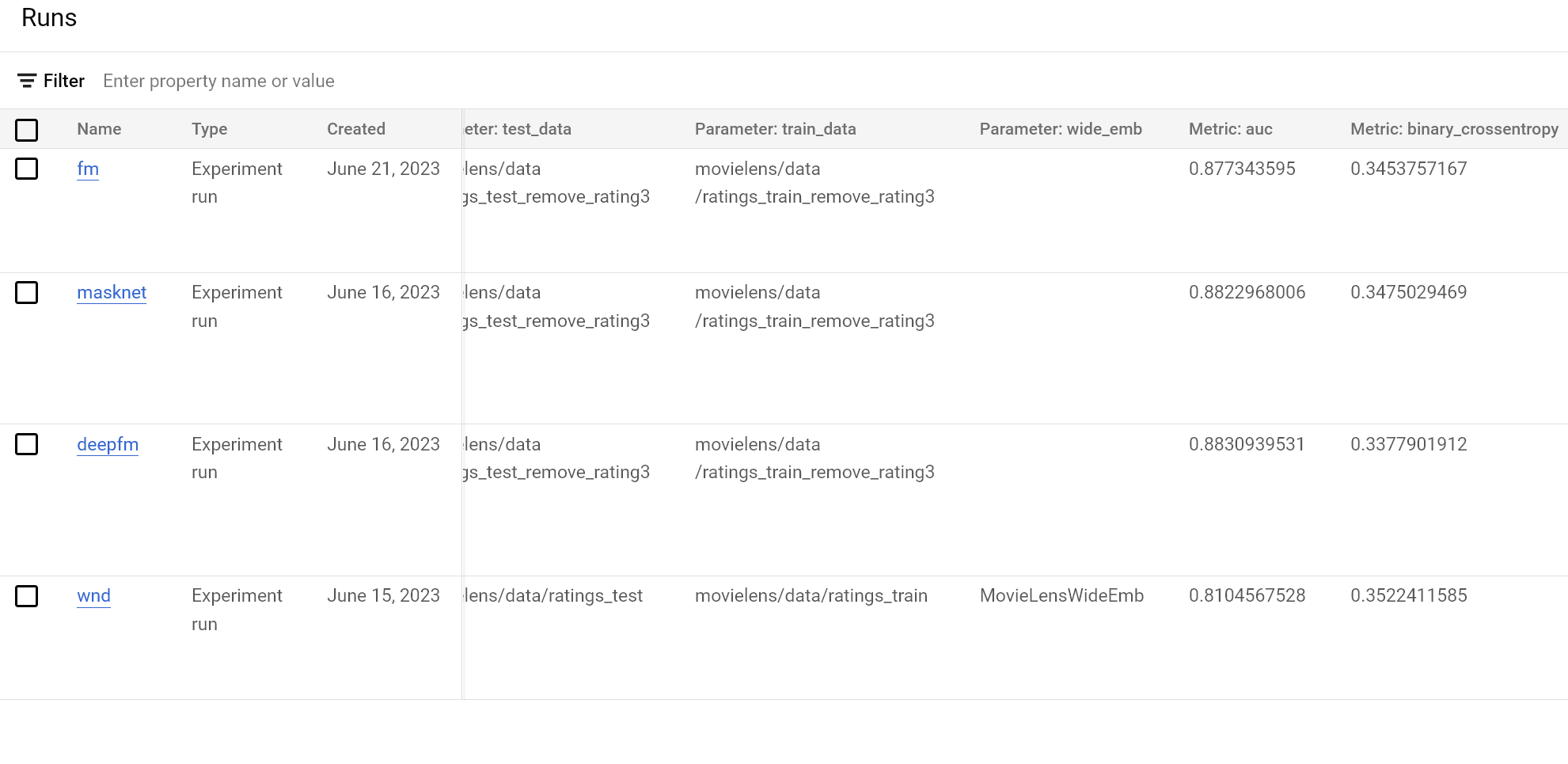
Train the above models on MovieLens 1m dataset (I use similar hyperparameter configs for all models without much tuning):
DeepFM and MaskNet is slightly better than FM, empowered by the Deep NN layers
W&D performs worst because I only do limited work on feature engineering
Weekly Digest
My 20 Year Career is Technical Debt or Deprecated, a fun story about how the techniques evolve.
The Curse of Recursion: Training on Generated Data Makes Models Forget, What will happen to GPT-n once LLMs contribute much of the language found online?
Sequential Testing at Booking.com, a practical guide on how booking leverage Sequential Testing to make reliable and fast product decisions. We don’t have to wait for the the required sample size arrives anymore.
A major benefit of sequential testing is that it does allow for interim analyses while maintaining the correct alpha error rate.
Mosh, a remote terminal application that allows roaming, supports intermittent connectivity, and provides intelligent local echo and line editing of user keystrokes.
https://nowave.it/factorization-machines-with-tensorflow.html
https://arxiv.org/pdf/1703.04247.pdf
https://zhuanlan.zhihu.com/p/58160982
https://zhuanlan.zhihu.com/p/456982760
Thanks for this great post.
I have 2 questions:
1. In your implementation of the FM layer (https://github.com/caesarjuly/reginx/blob/master/trainer/models/common/feature_cross.py#L25), there are no dense feature values used. It seems dense features are represented as embeddings, but their values are not used here. I'm not sure if I missed something. If I'm wrong, how are the values of dense features used?
2. If my understanding is correct, the final user embedding and item embedding are `concat_user_vector` and `concat_item_vector` (https://github.com/caesarjuly/reginx/blob/master/trainer/tasks/generate_fm_embedding.py#L53). And they are used in ANN matching as CR. I'm curious how important `item_score` is in the final embedding matching?
thanks.