
Quick data preprocessing with Pandas on Criteo Ads click data
A guide on how to analyze, format and handle open-source dataset

Start from today, besides academic papers, I will also write practical guides and tutorials on Machine Learning coding. I hope this can help our readers in their daily work. I cannot guarantee the frequency of updates for this type of article at the moment. Let’s try it first.
Criteo 1TB click logs dataset is one of the most popular open-source datasets for model evaluation. The training dataset consists of a portion of Criteo’s traffic over a period of 24 days. There are 13 features taking integer values (mostly count features) and 26 categorical features. Famous models like DLRM and DCN V2 all use this dataset as the experiment baseline.
When I try to reproduce the experiment results in the DLRM paper. I realize MovieLens data cannot meet our requirements because of the lack of dense features and the small size of training samples. So I start to prepare the Criteo data.
I take the first 7 days as the training set and randomly sample 10% from the 8th day as the validation set. I don’t have any distributed data processing framework like Spark at hand. So I use only Linux commands and pandas to finish the job.
I put all the code in my GitHub repository. It’s too big to show on GitHub, we can use a third-party tool to visualize it.
Task Description
The goal of the task is to generate a well-formatted dataset for training on TensorFlow. This includes 4 steps:
Data analysis and preprocessing, including scaling and data imputation
Downsampling the negative samples, to reduce training costs and have a balanced dataset
Build meta info, extract mean and variance from dense features for normalization, and generate vocabulary from sparse features for embedding table lookup
Generate the raw training and validation samples, typically we have 3 options:
Use CSV format, which can be directly exported from Pandas but this is inefficient considering loading speed and file size
Transformed to TFRecord, this can be done with the pandas-tfrecords library. But it requires trivial data schema parsing when loading. An example can be found here.
Directly load the data from Pandas to a TensorFlow dataset and leverage the save and load API to export and import the data. The APIs support sharding and compression which provides fast loading speed and small disk space usage. And it also saves the schema information together with the raw data, so we can skip the schema parsing part when loading the data for training. I will use this option here.
Data Analysis and Preprocessing
Visualize the data
For reference, many operations I used here follows the guide here.
Load and name the columns.

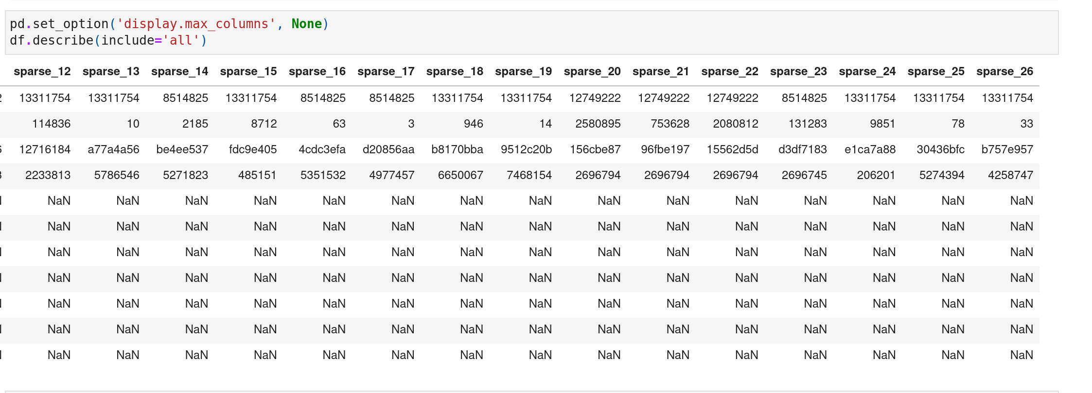
Check the general description. Here we can see that for the dense features, there are missing values NA and the value range varies a lot. And for dense_8, the min value is -1.0 which doesn’t make sense and could be a mistake.

For the sparse features, there are also many missing values and the vocabulary size differs.
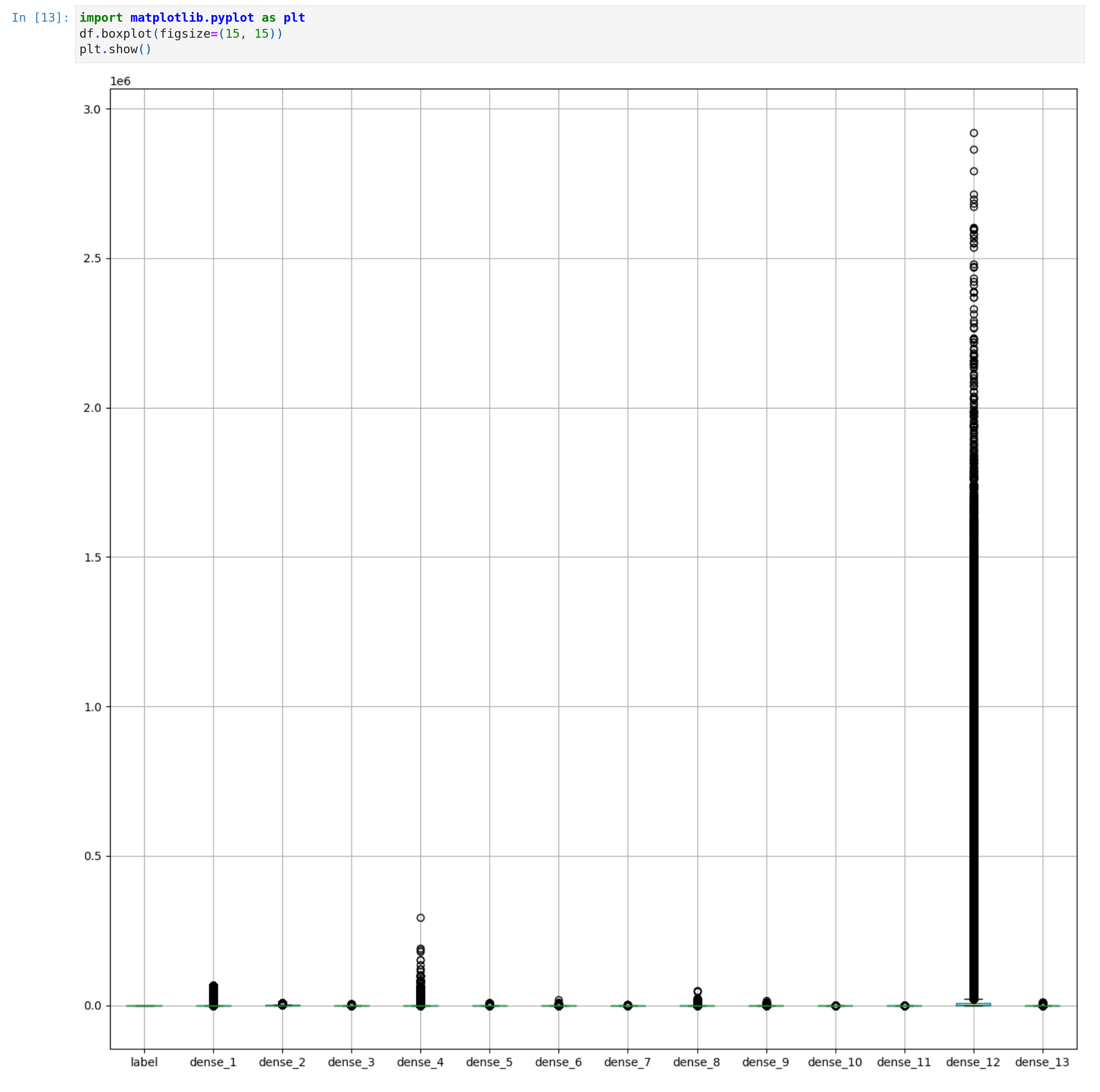
Next, let’s check the feature distribution. A helpful tool is the box and whisker plots.
A boxplot is a standardized way of displaying the dataset based on the five-number summary: the minimum, the maximum, the sample median, and the first and third quartiles.
We can see the value range is big, there all many outliers and the box can be barely seen. Especially for the dense_12, the value is much bigger than others. This means we should scale the values here.
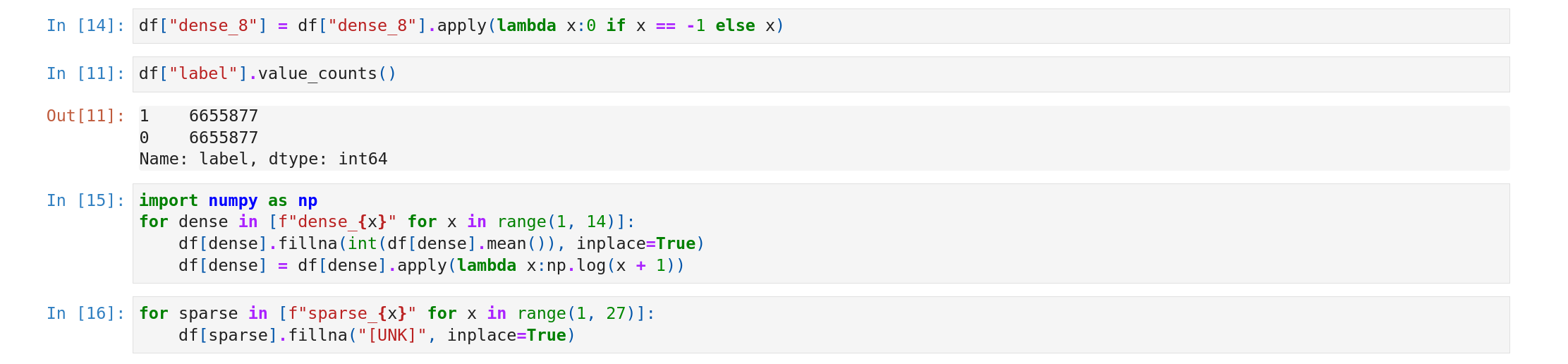
Replace the abnormal value in dense_8. Scale all the dense features using a logarithm. And also fill in the NA values with mean for dense features and [UNK] token for sparse features. Note that it’s better to use an unknown token [UNK] than the mode for sparse features here. This is because the unknown token can be learned as a separate embedding.
Check the boxplot again. Now it’s much better. Although there are still many outliers, especially for dense_7, we can also replace the outliers with the upper bound of the whiskers. Here I will just skip these extra steps.

Feature Distributions
Check the distribution of dense features. Now the value range is more reasonable. Note that the dense_10 feature is discrete and there are 3 buckets, this means we can try to discretize and split it into several bins. Also for the dense_7 feature, most values lie in a small range near 0, we can drop the bigger outliers.

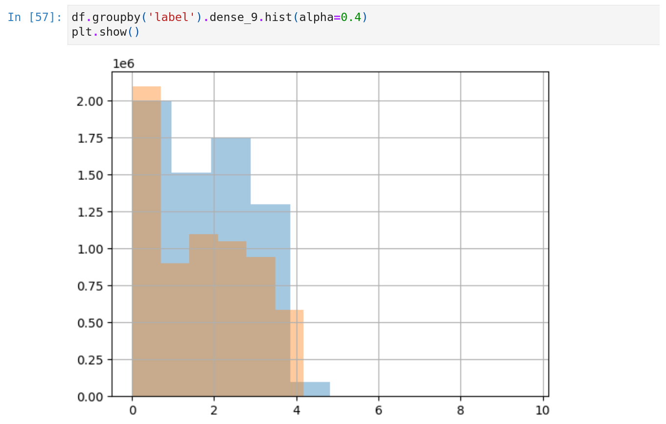
We can also check the feature-class relationships by generating a matrix of histograms for each attribute and one matrix of histograms for each class value.
This will generate 2 images. One for label 0, and the other for label 1. This helps us to figure out the difference in the distributions between the classes.
We can also plot the images on the same canvas for better contrast. We can see a distribution shift on the dense_9 feature, which means this feature can be helpful in discriminating the classes.
Feature Relationships
We can use the scatter_matrix to review the relationships between each pair of features.
This uses a built function to create a matrix of scatter plots of all attributes versus all attributes. The diagonal where each attribute would be plotted against itself shows the Kernel Density Estimation of the attribute instead.
For KDE, we can refer to this great illustration for better understanding.
In the below picture, notice that dense_5 and dense_11 are highly positively correlated, which means one of them can be redundant.

Downsampling
The original dataset is huge, approximately 40GB and 100 million per day. The positive and negative ratio is around 1:15. Our target metrics are AUC and LogLoss for binary classification, and AUC is insensitive to the number of negative samples. To achieve fast training, we simply downsample the negative samples to a 1:1 positive and negative ratio.
Here we use native shell scripts which are at least 10x faster than pandas operations.
#!/bin/bash
in=$1
in_gz="${in}.gz"
# download and unzip
mv ~/Downloads/$in_gz .
gzip -d $in_gz
# get positive numbers
awk '$1==1' $in > pos
pos_count=($(wc pos))
awk '$1==0' $in | shuf -n $pos_count > neg
# concatenate and shuffle
cat pos neg | shuf >"${in}_11"
Build Meta Info
The describe operator in Pandas already provides most of the meta info we need. But we also need to add the vocabulary info for the sparse features. Notice here we intentionally put the [UNK] token to the first index of the vocabulary list. This is the default oov_token for the TensorFlow StringLookup layer.

Generate Training Dataset
The final step is to load and save the data to a TensorFlow compatible format. The first option directly loads the data frame to the dataset but this will explode the memory usage. For big data like Criteo, it’s better to save and reload the data using the make_csv_dataset API. This API will build a generator and the memory usage is minimum.
Then we can use the tf.data.experimental.save API to shard, compress, and save the whole dataset. For the latest TensorFlow version, the save API has already been migrated to Dataset.save.
Notice that for the shard_func, we must use the tf.random API instead of Python or Numpy random. This is because, in the TensorFlow graph execution, the native Python or Numpy random operator will be calculated and included before the real execution. Hence, all the random values will be the same. This is also called a Closure.
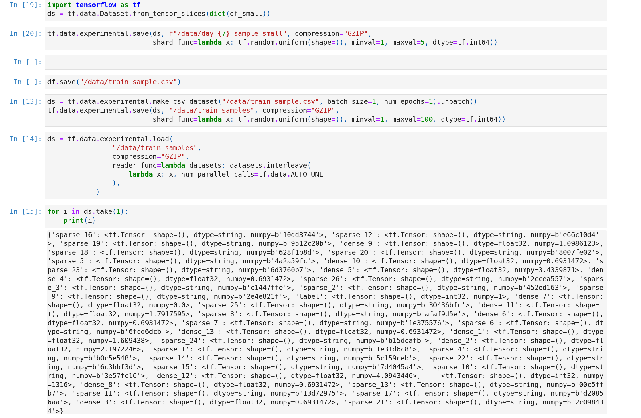
That’s it. Now we can use the dataset.load API to directly load the data while training. No schema parsing is required :).
