

Today let’s revisit one of the most classic papers in recommendation domain.1 In this paper, YouTube team
Introduces the standard structure of online recommendation system, candidate generation → ranking
Poses recommendation as extreme multiclass classification and verify effectiveness of negative sampling
Shares the detailed model structure and feature engineering work for candidate generation and ranker. The candidate generation model becomes the prototype of two-tower model
Covers the subtle details of how to handling practical problems like video freshness, data sampling and watch time weighted loss

Paper reading
Since this paper is so classic, most people are already familiar with it. Let’s change the way of read it. Here I only talk about the hightlights and tricky points.
Recommendation as Classification
Training
YouTube turns the prediction problem to accurately classifying a specific video watch wt at time t among millions of videos i (classes) from a corpus V based on a user U and
context C
🤔 Every video becomes a class, how YouTube handling the extreme multiclass problem in such a huge corpus?
To efficiently train such a model with millions of classes, we rely on a technique to sample negative classes from the background distribution (“candidate sampling”) and then correct for this sampling via importance weighting
The answer is negative sampling, here they don’t share much details on how to do the sampling. In general, I think they are build negative samples before training. Also they verify that hierarchical softmax performs poorly
Serving
For serving, they turns it to a ANN search issue - compute the most likely N classes (videos) in order to choose the top N to present to the user.
Here as they mentioned, they are using search algorightms like LSH to do this job. Also they found that A/B results were not particularly sensitive to the choice of nearest neighbor search algorithm.
Comine the training and serving pattern together, this becomes a standard approach for model candidate retriever like two tower.
Model architecture
Inspired by continuous bag of words language models we learn high dimensional embeddings for each video in a fixed vocabulary and feed these embeddings into a feedforward neural network

Video embedding
🤔 We can easily figure out that the user vectors are extracted from the last layer of the model. But how they generate the video embeddings?
Actually the video embeddings are the weights of the input layer of softmax function. For example, suppose the last hidden layer represents the user embedding, there are 2m output nodes represents the videos, then the dimension of the fully connected layer weights between user and videos are [100, 2m]. And the weight for a single output node is [100, 1]. This is exactly the embedding for a single video. When calculate the similarity, we can simply use the dot product of the u*v . The user and video embeddings are in the same space.
Example age
🤔 User prefer fresh content, how to introduce this feature to model?
In the paper, they feed the age of the training example as a feature during training. At serving time, this feature is set to zero (or slightly negative) to reflect that the model is making predictions at the very end of the training window.
We can see that after adding this feature, model can fit the distribution much better.

This is also the basic method to handle position bias in modern recommendation models.
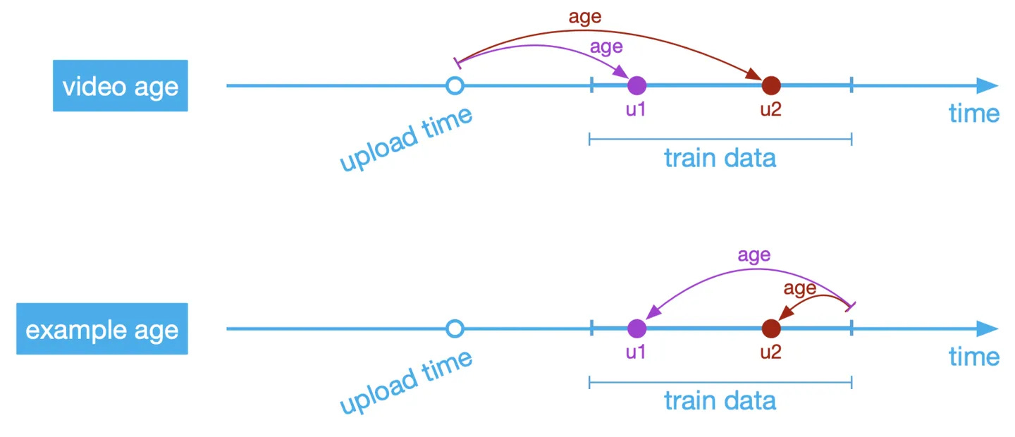
But here comes another question, why they don’t use video upload age? 🤔
The answer is actually quite simple.
Video age is equivalent to example age, their sum is a const2


In this paper, the only feature be used in video side is the ID. So there is no side info. The only choice left is add the age info to user side. If we use video age, then the user embedding is depend on video age, for each video we have to re-calculate the user embbedding. This is very expensive especially for online serving
Another implicit requirement is the video embedding should be relatively static. If use video age, it’s always shifting which make it hard for serving
User based sampling
Another key insight that improved live metrics was to generate a fixed number of training examples per user, effectively weighting our users equally in the loss function.
🤔 Why only choose fixed samples for each user, not from all the samples?
This prevented a small cohort of highly active users from dominating the loss.
Drop sequential information
In this paper, they intentional withhold information from the classifier, only use average pooling for all the user histories, 🤔 why?
a classifier given this information will predict that the most likely videos to be watched are those which appear on the corresponding search results page for “taylor swift”.
This problem is already solved by modern sequential models like GRU or Transformer. And we already proved that the sequential information is critical. And YouTube also applied 3 to their system.
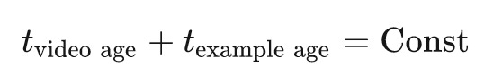
Predicting future watch
YouTube choose to use future watch as the predicting label instead of held-out watch, 🤔 why?
Episodic series are usually watched sequentially and users often discover artists in a genre beginning with the most broadly popular before focusing on smaller niches
This approach prevents data leak. This discussion from the paper actually also shows that the sequential information is critical.
Weighted LR
🤔 Why use weighted LR as the training label and use e(Wx+b)4 as the serving score? This is the most interesting design in this paper.
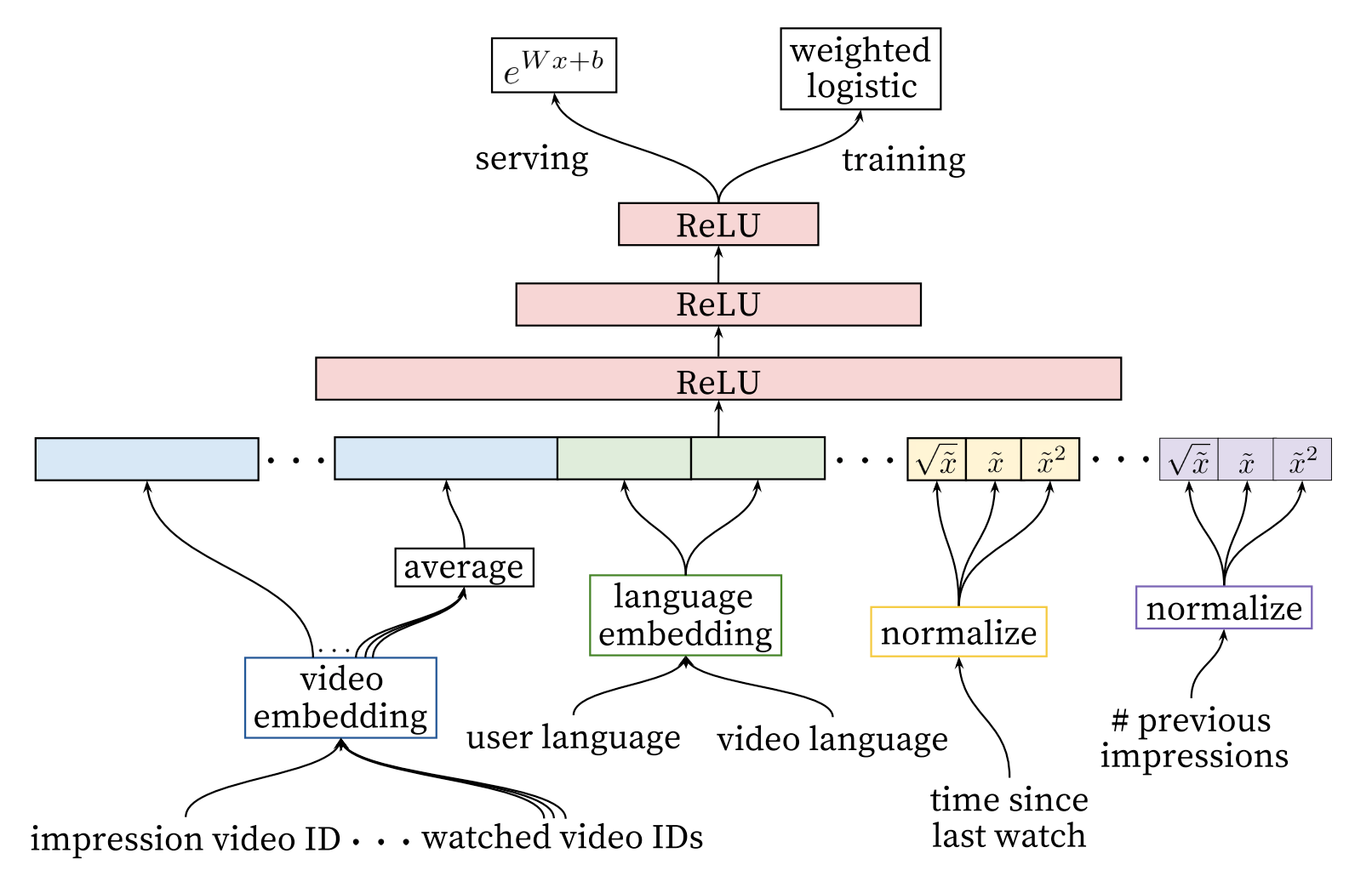
However, the positive (clicked) impressions are weighted by the observed watch time on the video. Negative (unclicked) impressions all receive unit weight.
Then they get the odds are close to the expected watch time.
the learned odds are approximately E[T ](1 + P ), where P is the click probability and E[T ] is the expected watch time of the impression. Since P is small, this product is close to E[T ].
But how? According to the definition of LR, We know that odds is equal to 5
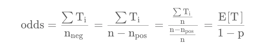
Then based on Taylor expansion
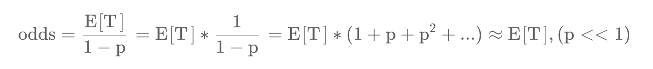
Then the odds is
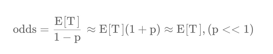
One strange thing here is YouTube assume the P is small, so actually 1/(1-p) is approximate to 1, there is no need to do a Taylor expansion.
Another thing is P is not that small, we know that commonly the click rate of video can be around 10% or larger, how can we ignore this directly?
My example
Let’s see my concrete example on weighted LR.
YouTube doesn’t open their dataset to public, so I use Movielens’ data as the baseline.
Since Movielens data doesn’t have negative samples, so I randomly generate negative samples from the whole corpus.
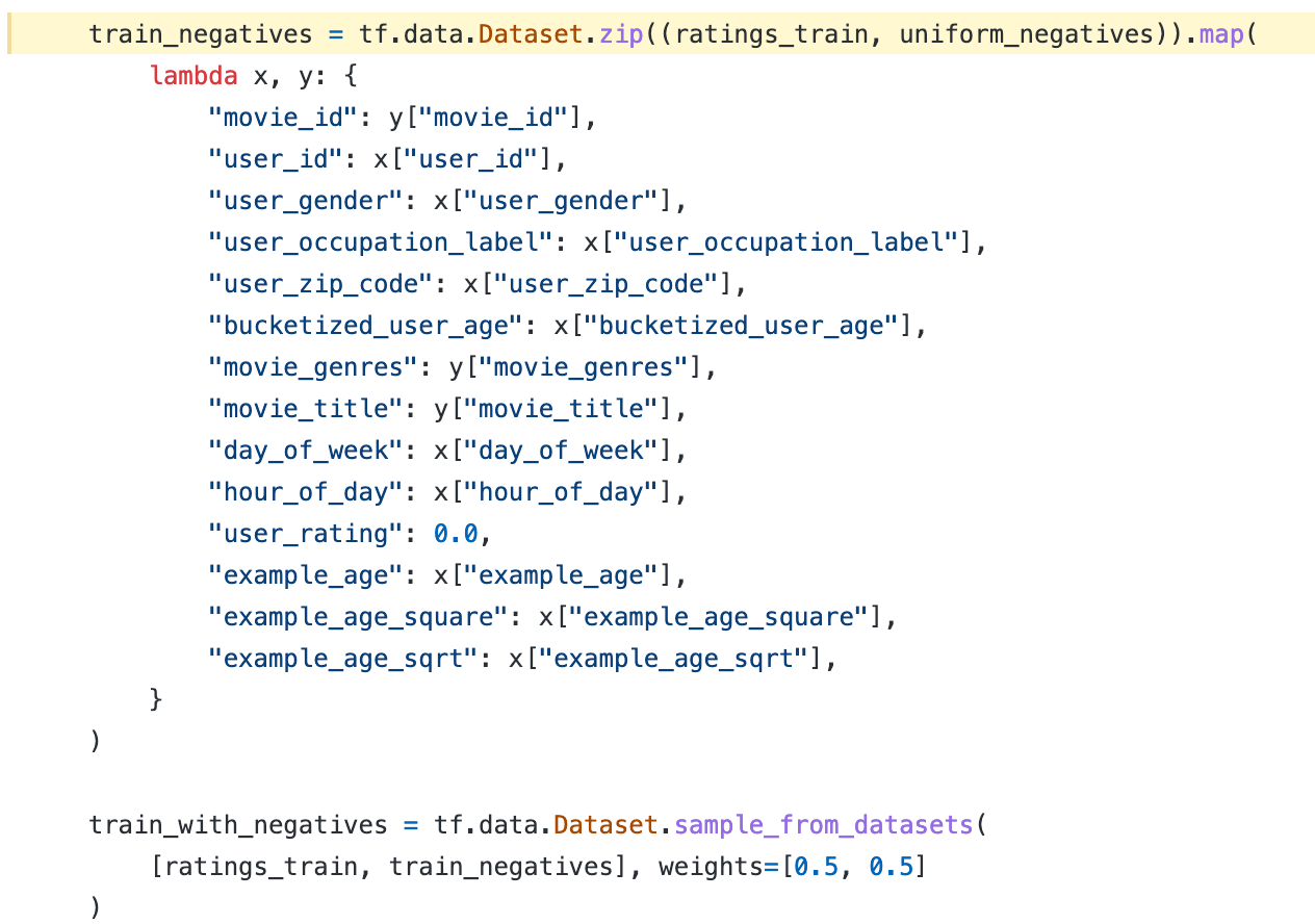
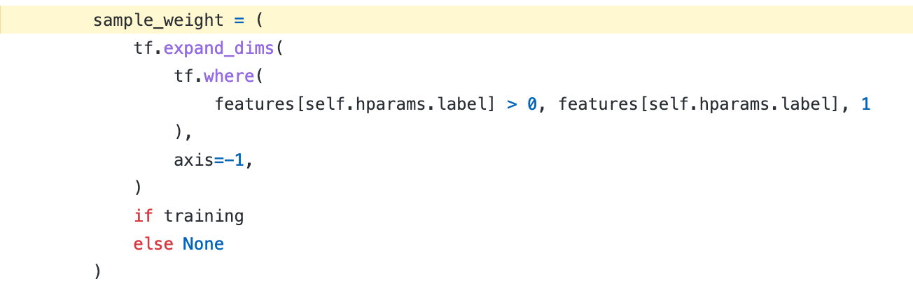
For example age, I use a simplified min_max scaler for the feature preprocessing.

Then for the training part, I use the user_rating score as the sample weight, this is similar to use watch time.
The model structure is same as the paper.
Train it for 2 epochs and we have a OK baseline with metrics as

Let’s pick 10 samples to verify the prediction results.
[0. 2. 5. 0. 0. 0. 3. 4. 3. 0. 0. 4. 4. 3. 3. 2. 5. 0. 0. 2.]And the corresponding predict result. Note that the result is not perfect. Some zero score rating still have high score.
[0.0037087505, 0.96394616, 0.8644594, 0.6511643, 0.9675827, 0.8655438, 0.9078593, 0.9634518, 0.945095, 0.62273407, 0.90941566, 0.5690908, 0.9706214, 0.9304068, 0.9185634, 0.28620714, 0.48636842, 0.8152434, 0.98603284, 0.9709172]In order to get the odds, we need to do 2 extra steps
Calibration, since our negative samples are not the real distribution. Suppose the real CTR is around 10%.
Reverse sigmoid, get the numbers before sigmoid layer

list(map(lambda x:math.trunc(math.exp(reverse(calibrate(x)))), a))
[0, 2, 0, 0, 2, 0, 0, 2, 1, 0, 1, 0, 3, 1, 1, 0, 0, 0, 7, 3]
As we can see here, for the precise predictions the result is close to the original rating, aka the expected watch time.👏
Weekly digest
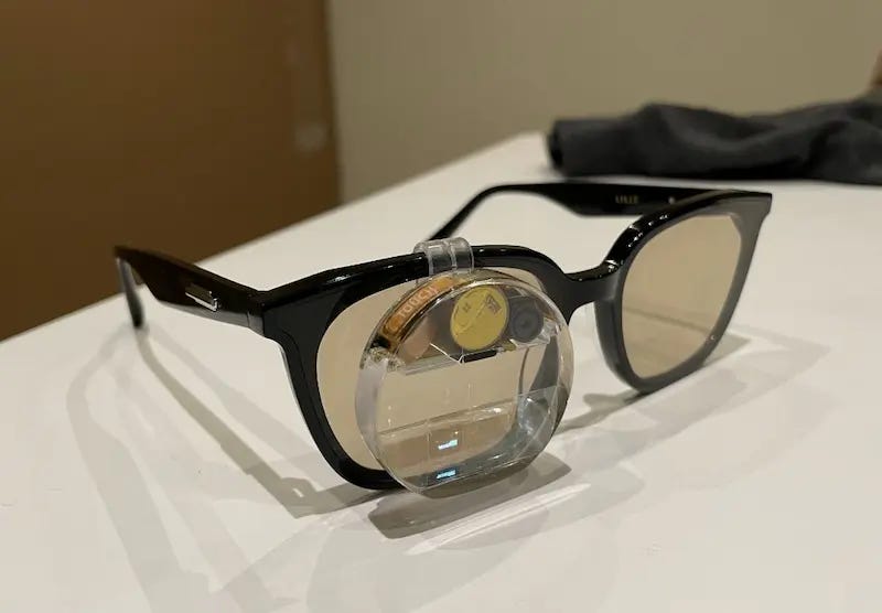
ChatGPT glass, embed ChatGPT to your glass!

A brief introduction of twitter’s recommender system from SAI
Meta’s new model segment-anything, a new AI model from Meta AI that can "cut out" any object, in any image, with a single click
The Anti-Productivity Manifesto. The central premise of the book is simple: everyone has got about four thousand weeks to live, and spending that limited time chasing efficiency is wrongheaded
Cheating is all you need. There is something legendary and historic happening in software engineering, right now as we speak, and yet most of you don’t realize at all how big it is
Treat your to-read pile like a river, not a bucket. The real trouble, according to the leading techno-optimist Clay Shirky, wasn't information overload, but "filter failure"
Remembering Bob Lee. Thank you, I'll miss you 'crazybob'.

What’s next
Twitter’s recommendation algorithm is super interesting. I will go through it in the next few posts.
https://static.googleusercontent.com/media/research.google.com/en//pubs/archive/45530.pdf
https://zhuanlan.zhihu.com/p/372238343
https://static.googleusercontent.com/media/research.google.com/en//pubs/archive/46488.pdf
https://zhuanlan.zhihu.com/p/52504407
https://blog.csdn.net/ggggiqnypgjg/article/details/108968483