Optimization in Multi Task Learning I

Understand and implement popular multi task optimizers

Today let’s continue our learning on multi task models. From now on, I will write a series of posts about multi-task optimization approaches. This post will talk about the uncertainty weighting and gradient norm approaches first. (I find it’s too long to introduce all the approaches in one post)

I learned these methods mainly from a survey paper¹ published on 2021. In the recent two years, there are new progresses on this topic. I will read and summarize the latest progress soon.

Task Balancing Approaches

Introduction

First let’s introduce basic formulas to help us understand why optimization in MTL is important.

The optimization objective in a MTL problem, assuming task-specific weights w_i and task-specific loss functions L_i, can be formulated as:

\(L_{MTL} = \sum_iw_i*L_i\)

If we use stochastic gradient descent to minimize the objective, the network weights in the shared layers W_sh are updated by the following rule

\(W_{sh} = W_{sh} - γ\sum_iw_i\frac{\partial L_i}{\partial W_{sh}}\)

From this equation, we can see:

1. The network weight update can be suboptimal when the task gradients conflict, or dominated by one task when its gradient magnitude is much higher w.r.t. the other tasks

2. Each task’s influence on the network weight update can be controlled, either indirectly by adapting the task-specific weights w_i in the loss, or directly by operating on the task-specific gradients

Uncertainty Weighting

The uncertainty weighting approach uses task-dependent or homoscedastic uncertainty to balance the single-task losses².

Homoscedastic Uncertainty

What is homoscedastic uncertainty? It’s a quantity that remains constant for different input examples of the same task. This concept comes from Bayesian modelling and I find it hard to understand without knowing the statistic theory. Let me quote some explanation from this post for clarification.

Epistemic uncertainty describes what the model does not know because training data was not appropriate. Epistemic uncertainty is due to limited data and knowledge. Given enough training samples, epistemic uncertainty will decrease. Epistemic uncertainty can arise in areas where there are fewer samples for training.

Aleatoric uncertainty is the uncertainty arising from the natural stochasticity of observations. Aleatoric uncertainty cannot be reduced even when more data is provided. When it comes to measurement errors, we call it homoscedastic uncertainty because it is constant for all samples. Input data-dependent uncertainty is known as heteroscedastic uncertainty.

The illustration below represents a real linear process (y=x) that was sampled around x=-2.5 and x=2.5.

An exhibit of the different kinds of uncertainty in a linear regression context (Image by Michel Kana).

1. Noisy measurements of the underlying process lead to high aleatoric uncertainty in the left cloud. This uncertainty cannot be reduced by additional measurements, because the sensor keeps producing errors around x=-2.5 by design

2. High epistemic uncertainty arises in regions where there are few or no observations for training

In simple words, we can think of homoscedastic uncertainty as a measure of inherent task noise.

The optimization procedure is carried out to maximise a Gaussian likelihood objective that accounts for the homoscedastic uncertainty. Remember that in Gaussian maximum likelihood estimation, the method estimates the parameters of a model given some data using Gaussian distribution.

Also according to this post, the variance can be seen as a measure of uncertainty and it’s the sum of the aleatoric and epistemic uncertainty.

Therefore in this paper, the noisy level of the task, defined as the variance in Gaussian distribution, can be turned into the loss weight to modeling the homoscedastic uncertainty.

Derive the Multi-Task Loss Function

Let me show the example on the regression task. For the classfication task, it’s a similar process and you can refer to the paper for details.

Let f(x) be the output of a neural network with weights W on input x. We define our likelihood as a Gaussian with mean given by the model output and with an observation noise scalar σ.

\(p(y|f^W(x)) = \mathcal{N}(f^W(x), \sigma^2) = \frac{1}{\sqrt{2π\sigma^2}}e^{-\frac{1}{2\sigma^2}(y-f^W(x))^2}\)

For multiple model outputs, we often define the likelihood to factorise over the outputs with model outputs y_1, ..., y_K.

\(p(y_1, ..., y_K |f^W(x)) = p(y_1|f^W(x))...p(y_K |f^W(x))\)

In maximum likelihood inference, the log likelihood for a Gaussian likelihood with σ the model’s observation noise parameter can be written as:

\(log p(y|f^W(x)) ∝ − \frac{1}{2σ^2} ||y − f^W(x)||_2 − log σ\)

Assume that our model output is composed of two vectors y_1 and y_2, each following a Gaussian distribution.

\(p(y_1, y_2|f^W(x)) = p(y_1|f^W(x)) · p(y_2|f^W(x)) = N (y_1; f^W(x), σ^2_1 ) · N (y_2; f^W(x), σ^2_2 )\)

We can get the final minimisation objective as:

\(− log p(y_1, y_2|f^W(x)) ∝ \frac{1}{2σ^2_1} ||y_1 − f^W(x)||_2 + \frac{1}{2σ_2^2}||y_2 − f^W(x)||_2 + log σ_1σ_2\)

Represent the loss of the output variable as L(W), the above equation equals to:

\(L(W, \sigma_1, \sigma_2) = \frac{1}{2\sigma_1^2}L_1(W) + \frac{1}{2\sigma_2^2}L_2(W) + log(\sigma_1\sigma_2)\)

We can see here, the σ_1, σ_2 noise parameters become the loss weight. Note that:

1. As σ_1 the noise parameter for the task1 increases, we have that the weight of L_1(W) decreases

2. As the noise decreases, we have that the weight of the respective objective increases

3. The noise is discouraged from increasing too much (effectively ignoring the data) by the last term in the objective, which acts as a regularizer for the noise terms

4. This is advantageous when dealing with noisy annotations since the task-specific

   weights will be lowered automatically for such tasks

5. We can find that uncertainty weighting prefer easy tasks (low noise)

Implementation

The implementation is straightforward. We just need to define the two σ as the trainable weights. Notice that there is a trick, instead of directly learn the σ in the equation. We take the trainable variable as the log variance log(σ^2) and use exponential operation to map it back for numerical stability. This can avoids any division by zero.

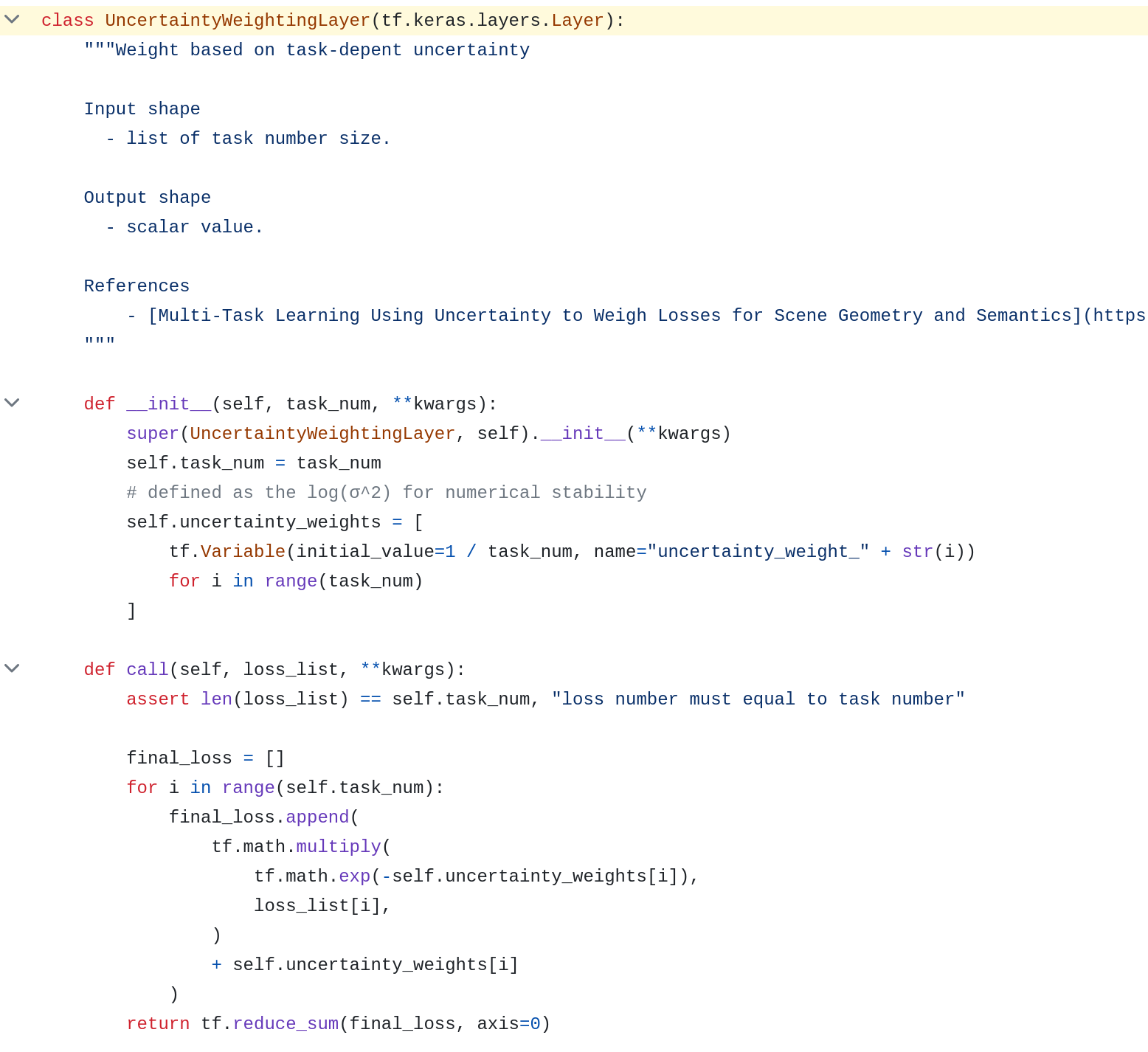
When training the model, just pass the loss list to this layer and it will calculate the final loss for you.

Gradient Normalization

Gradient normalization (GradNorm) proposed to control the training of multi-task networks by stimulating the task-specific gradients to be of similar magnitude and learning pace.

To understand this approach, we need to define a few notations first:

1. The L2 norm of the gradient for the weighted single-task loss w_i (t) · L_i (t) at step t w.r.t. the weights W

   \(G_i^W(t) = ||\nabla_Ww_i(t)L_i(t)||_2\)

2. The mean task gradient averaged across all task gradients w.r.t the weights W at step t

   \(\bar{G}^W(t) = E_{task}[G_t^W(t)]\)

3. The inverse training rate of task i at step t

   \(\tilde{L}_i(t) = L_i(t) / L_i(0)\)

4. the relative inverse training rate of task i at step t

   \(r_i(t) = \tilde{L}_i(t)/E_{task}[\tilde{L}_i(t)]\)

GradNorm controls the gradient magnitude and learning pace by minimizing the following loss:

\(|G_i^W(t) - \bar{G}^W(t) \cdot r_i(t)|\)

1. The gradient maginitude is controlled by making the individual task gradient as close to the average as possible

2. The learning pace is controlled by the relative inverse training rate. When

   the relative inverse training rate increases (the task learns slower), the gradient magnitude for task i should increase as well to stimulate the task to train more quickly

Remember that the individual task gradient depends on the weighted single-task loss w_i (t) · L_i (t) . So the above loss can be optimized by adjusting the weight.

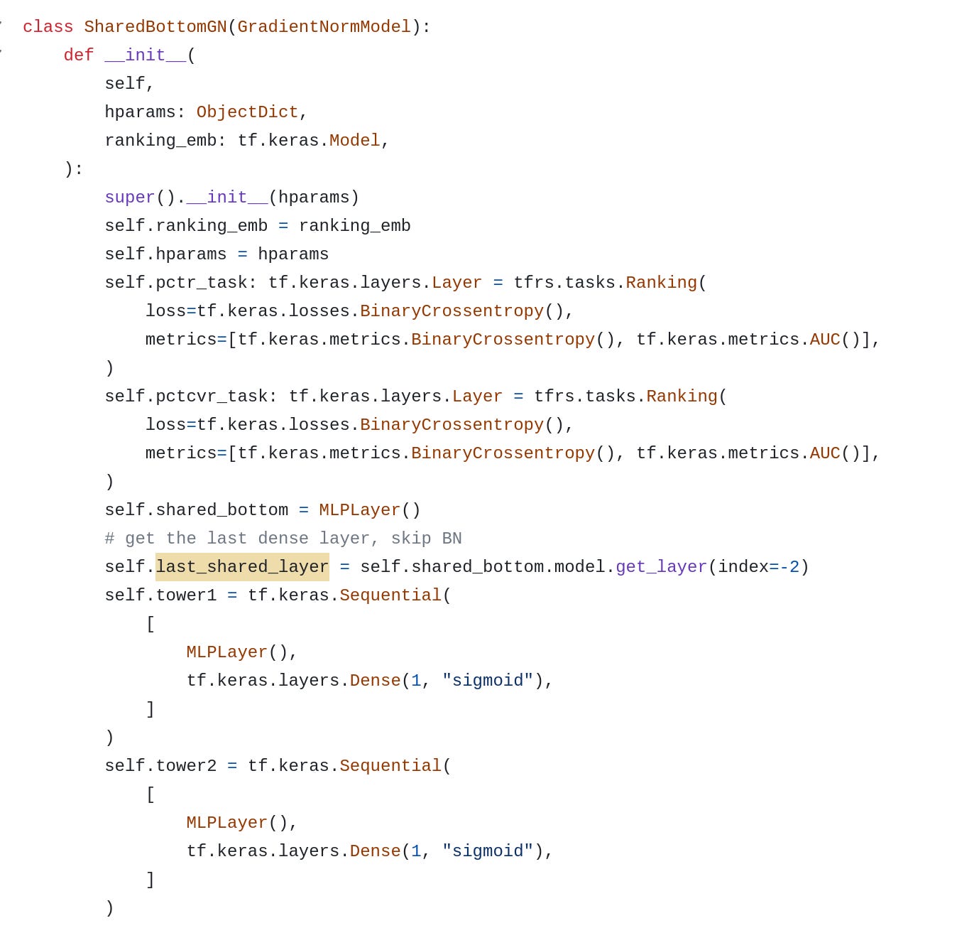
Note that, calculating the gradient magnitude requires a backward pass through the task-specific layers of every task i. We can save the computation time by only considering the gradient on the last shared layer.

Different from uncertainty weighting which uses task-depend uncertainty to re-weight the loss. And it prefers low noise task. GradNorm doesn’t have the concept of task priority, it only want to balance the gradient magnitude and learning pace.

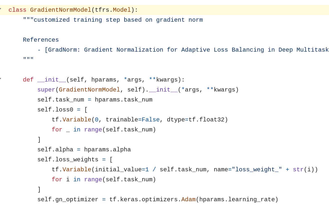
Implementation

Implement GradNorm in TensorFlow is a bit complicated. I tried my best to make it clear. I didn’t find any implementation for TensorFlow 2 yet, and I hope this can help us in our daily work.

First, we need to define the first step loss and the loss weight. We also need to create a separate optimizer for learning the loss weights. Because by default, TensorFlow 2 doesn’t the same optimizer to be used for separate weights.

Notice that here the we have to inherit the base model because the GradNorm requires us to customize the training step and manipulate the gradients.

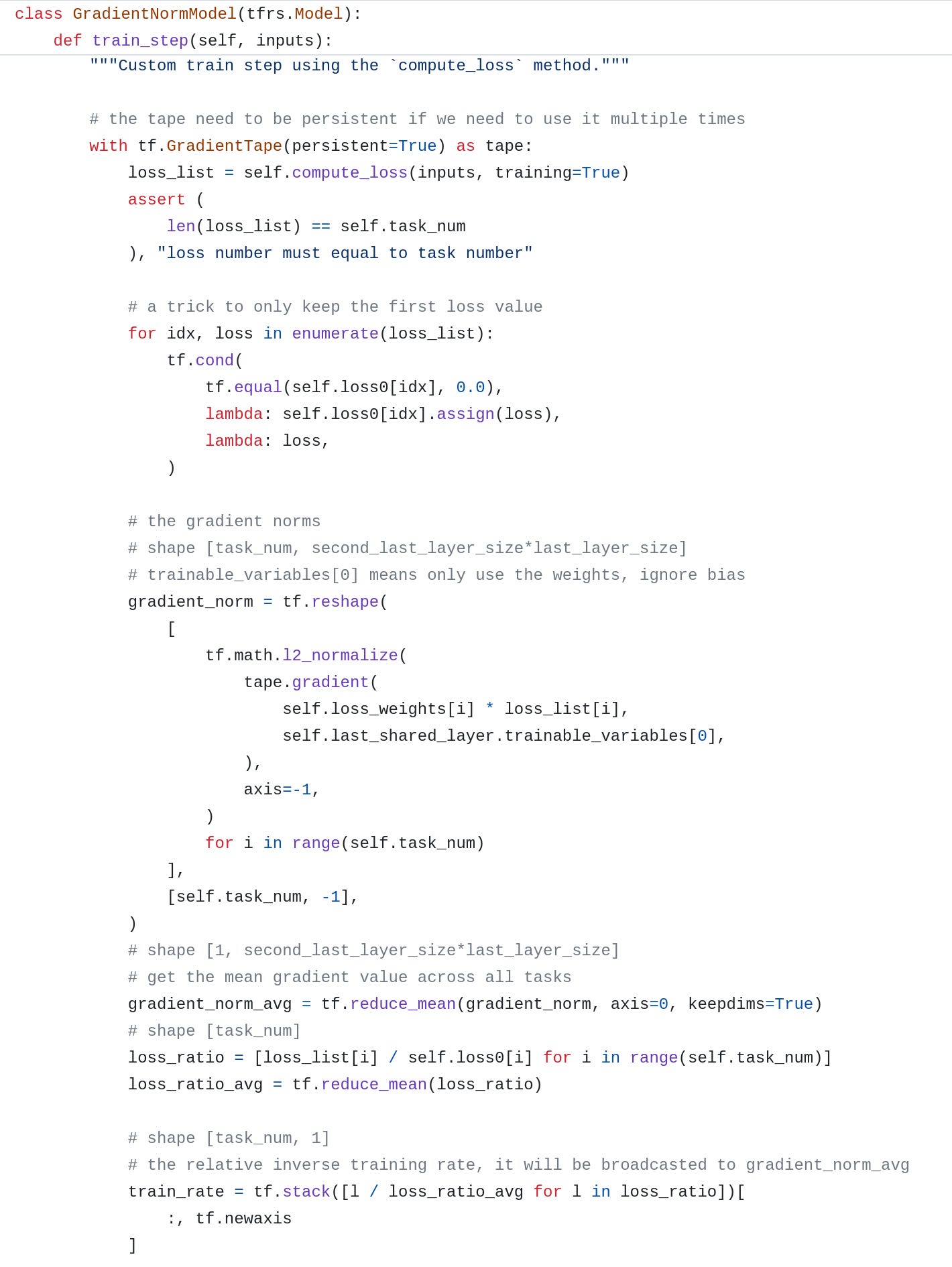
Then in the training step, first we need to create a persistent gradient tape for reuse. Then:

1. We pass in the loss list and use tf.cond to store the losses for the first step

2. Calculate the gradients for each task and normlize it. Without loss of generality, here we assume the last layer is a dense layer with [M*N] size

3. Reduce and calculate the average gradient across all the tasks

4. Calculate the relative reverse training rate based on the current loss and first-step loss

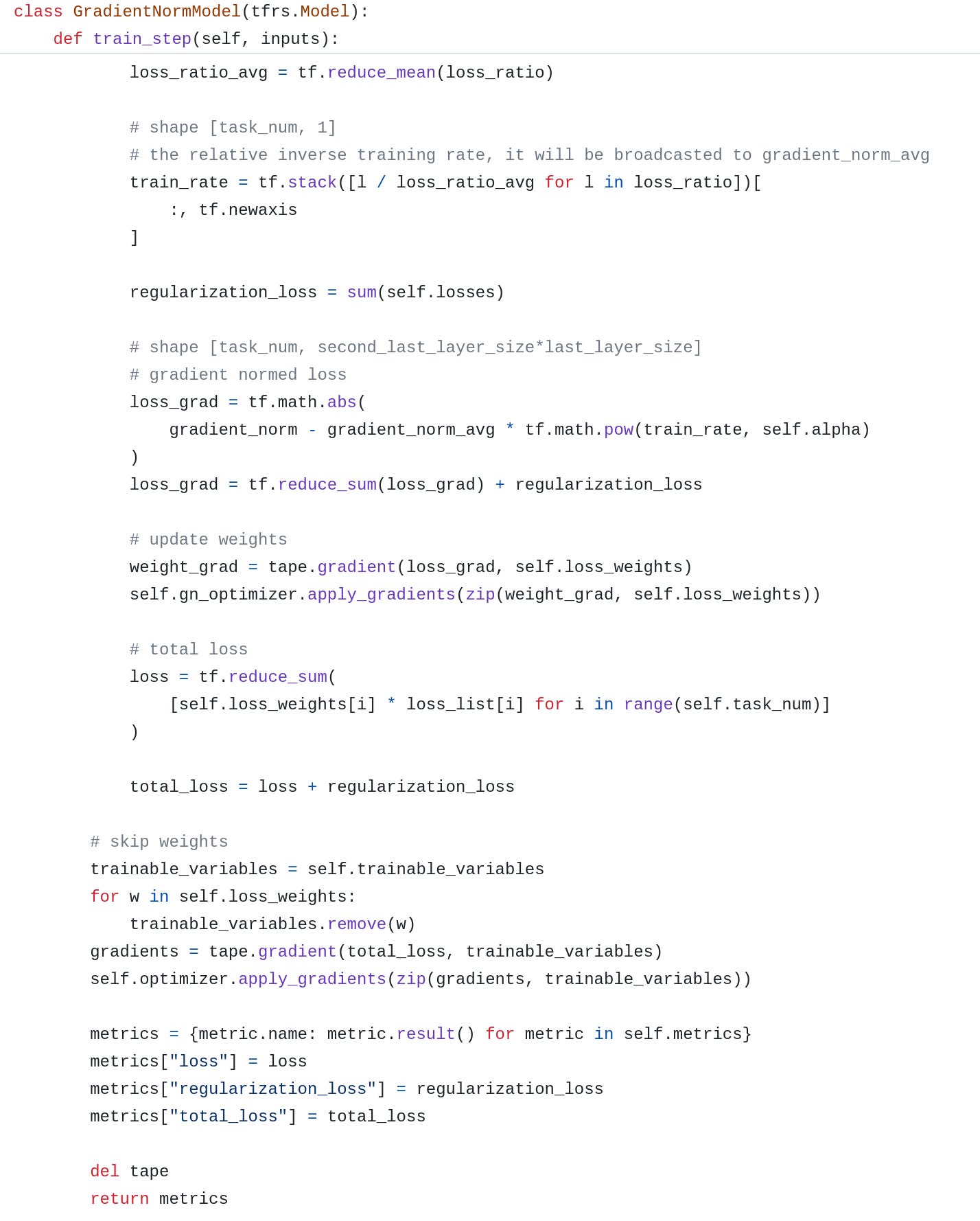
In the next step, we just follow the equation and calculate the objective loss for the gradient. Then update the weights using the gradients.

After updating the gradient, we need to remove the weights from the trainable_variables pool to avoid duplicated updating. Then we conduct a whole weights update on all the variables. Remember to manually delete the tape after finishing the whole training step.

In the training model, here I use a shared bottom model. Remeber to record the last shared layer. Then every thing is ready, just train it.

I also implemented other optimizers in this file. You can refer to it if you are interested. I will share the details in the next post. 📝

Recently I joined a startup company and I’m getting busier and busier. So I cannot guarantee to post new articles every week. I hope you guys can understand. 🙏

But I will persist in continuing to write. See you soon.

1. https://arxiv.org/pdf/2004.13379.pdf

2. https://arxiv.org/pdf/1705.07115.pdf