Two tower candidate retriever I

Bias correction for in-batch negative sampling

In this post, I will go through the classic two tower paper from google, aka Sampling-Bias-Corrected Neural Modeling for Large Corpus Item Recommendations¹, and show a concrete implementation example from TensorFlow Recommender.

Paper reading

Abstract

In the abstract, the author brings the issue we meet in industry recommendation system, retrieving and scoring items from a very large corpus. One common recipe to train a two-tower model is to learn the user and item representation and calculate loss functions from in-batch negatives. But in-batch loss is subject to sampling bias, especially in a highly skewed data distribution which is very common in industry. So the author bring a novel algorithm to estimate the item frequency from streaming data and verify the performance on YouTube.

Key points:

1. Very large corpus, makes it impossible to calculate a full softmax for all items in the corpus. Negative sampling is a must

2. Estimate from streaming data, this means the algorithm can adapt to the change of item frequency and be applied to real-time model training which is critical for modern recommender systems

Introduction

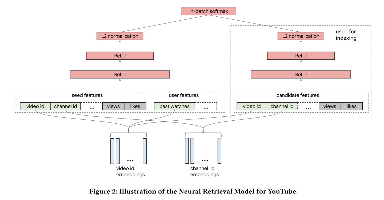
In this part, the author revisits the history of recommendation models and give a short introduction on two-tower model which is good at modeling <user, context> and <item> relationships, and incorporating rich user, item features.

As illustrated above, the left tower is a user tower, which normally input with user, context features, ingest these features with several layers of MLP and output the user vector. The right tower is a item tower, input with item content features and it has the same structure as the user tower.

The two-tower model is generalized from MLP models, like the YouTube DNN².

For the MLP models:

1. they are trained with many sampled negatives from the whole corpus

2. the item tower is simplified to a single layer with item embeddings. So it's fast to train

But for two-tower model:

1. the item tower is much more complex

2. not feasible to have a large amount of negatives

3. In batch softmax as the common solution, calculate the probability in a single batch

But in bach softmax is subject to sampling bias. Then the author bring up a novel algorithm to solve this issue.

Related work

In this part, the author mainly talks about the framework of two-tower model and explains the algorithm.

Estimate probability within a batch and optimize the loss

Because we are using in-batch negatives and the power-law distribution, the popolar items are over penalized. The logits need to be corrected by LogQ correction.

Normalization and Temperature

They found emperically, the performance can be improved by adding a normalization embedding normalization layer and a temperature hyper-parameter to scale the logits.

My comment 🤔: In my experience, this 2 params do have a big impact on the final performance, around 5% improvement on the recall rate metrics.

Streaming frequency estimation

In this part, the author gives a math proof of the algorithm and describe the steps.

δ denotes the average number of steps between two consecutive hits of the item.

A[h(y)] records the latest step when y is sampled, B[h(y)] contains the estimated δ of y

And they also prove that with as t → ∞, the bias will be 0. And the variance is limited by

Here δ = E(∆), t − A[h(y)] is a sample of ∆

Regarding the learning rate α

1. higher rate causes a faster decrease of the first term that depends on initialization error — converge faster, but be affected higher by the variance

2. lower rate reduces the second term which depends on the variance of ∆ and does not decrease over time — converge slower

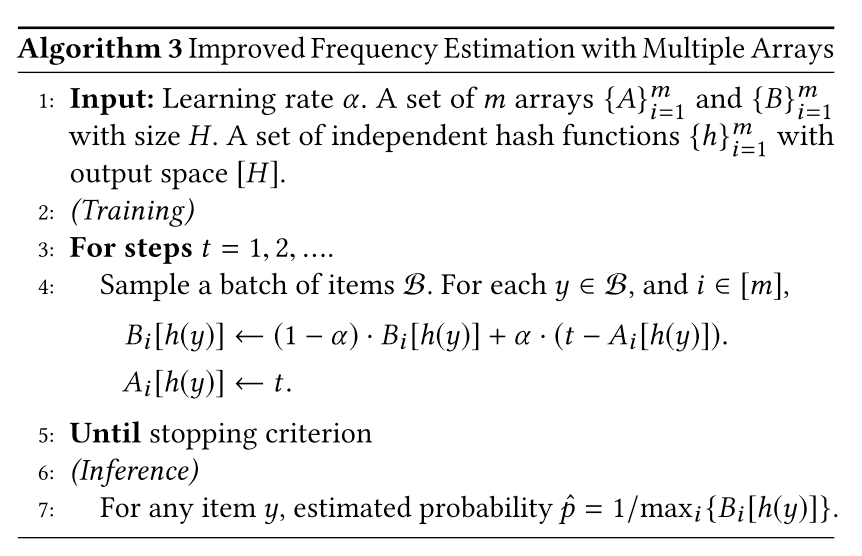
They also consider the hash collision and bring another upgraded algorithm 3 using multible hash functions. Then they take the maximum of multiple estimations representing the number of steps between two consecutive hits.

Each bucket in B could be an under-prediction of the true step gap as it could represent the union of multiple items because of collisions.

Neural retrieval system for YouTube

In this part, the author shares the detailed model structure and training strategy for YouTube

1. Training label, click weighted by watching complete ratio

2. Video features

   1. Dense features, normalization

   2. Categorical features

      1. One value, like video ID, one embedding as the representation

      2. Multiple values, like topic IDs, weighted sum of embeddings

      3. Out-of-vocabulary entities, randomly hashed to a bucket

User features

1. Current watching video as the seed video features, same features shared with item tower

2. Watch histories, average of the video embeddings

3. Embedding features are shared between the two tower

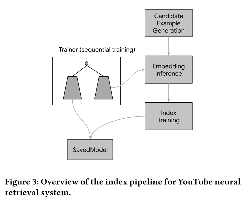
The training data is generated on a daily basis and feed into the trainer. The serving part is separated into 4 stages:

1. Select candidate video set based on the their business requirement

2. Use item tower to generate embeddings for all candidates

3. Train the index model for the generated embeddings, here probably they are using Google’s ANN library Scann³

4. For the last stage, they save the user tower together with the trained index and serve them online. My comment 🤔:

   1. In traditionally approach, people usually separate the user embedding online inference from the candidate index building

      1. The user tower will be saved and served for online real-time inference

      2. The item tower will be used for offline index generation. Then the index will be deployed separately for online search. This can be done leveraging ANN library like Faiss ⁴

      3. This approach has a consistency issue, there is a time gap between deploying user tower and index. This can be solved by add an additional version tag for both user and index model. When querying, specify the corresponding model using the tag. But this still bring more complexity

   2. In this paper, they avoid this issue by save and serving user and index model together. There is a concrete example in TensorFlow Recommender library

The index and user model are saved together

Experiments

In this part, the author conducts a few experiments to verify the performance of sampling bias correction. I picked the 2 most important tests here.

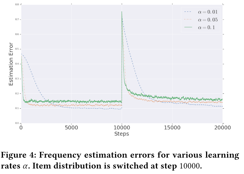
Simulation on frequency estimation

With a higher learning rate, the algorithm is more adaptive to distribution change, but the final variance is higher.

Switch the item distribution on 10000 step

YouTube Experiments

Model structure:

1. three-layer DNNs with hidden layer sizes [1024, 512, 128] for both
   towers

2. train the model using Adagrad, learning rate 0.2, and batch size 8192. My comment 🤔: Interesting to see they use a huge batch size with a large learning rate, guess the model size is not very big

3. for frequency estimation, they set H = 50M, m =1, α = 0.01

4. index of approximately 10M videos (this is large, need to use approximate search algorithm) chosen from the YouTube corpus is built periodically every few hours (few hours is not even near real-time, I guess this is because the engagement growth of new video is slower compared to news scenario)

Model training:

1. 15 days data training as the warm up phase

2. 10% data for evaluation

3. average 7 days results after the first 15 days

4. for in batch softmax, the offline result is significantly better than mse baselins (I doubt why choose this as the baseline, it’s quite weak)

5. corrected softmax is also significantly better than plain softmax

Online ab test:

1. for control group, no change. My comment 🤔: it will be much better if they share the details of the control settings

2. for treatment group, add the new model as a new candidate retriever

3. both versions show significant gain

Build a frequency estimation layer

Let’s build the sampling bias correction layer leveraging the experimental API from TensorFlow.

In the paper, they use a fixed length array to record the steps, then use hash functions to map the keys to the array index. Actually this is equivalent to a hashmap. Now TensorFlow provides the DenseHashTable and MutableHashTable data structure, we can build the algorithm on it.

Quick comparison between these 2 hash tables:

1. DenseHashTable offers generally faster insert, remove and lookup operations, in exchange for a higher overall memory footprint. This is because it has an aggressive momery allocation strategy . And it uses "open addressing" with quadratic reprobing to resolve collisions

2. MutableHashTable uses the standard C++ hash table API. So it doesn’t need to specify empty_key and deleted_key

3. In this case, I prefer faster query than memory consumption because in general we want to train faster. So I choose DenseHashTable

Here is the code

class SamplingBiasCorrection(tf.keras.layers.Layer):
    """A naive implementation of SamplingBiasCorrection.
    It supports the basic step estimation operation and returns the sampling probability for each key.
    Notice it doesn't support key expiration yet, so the memory will continue to grow if used in sequential training.
    """
    def __init__(self, lr=0.05, **kwargs):
        """Use one table to record the lastest step, aka the A table in paper
        Use another table to record the estimated step gap for each key, the B table in paper
        """
        super(SamplingBiasCorrection, self).__init__(**kwargs)
        self.lr = lr
        self.lastest_step = tf.lookup.experimental.DenseHashTable(
            key_dtype=tf.string,
            value_dtype=tf.int64,
            default_value=0,
            empty_key="",
            deleted_key="$",
        )
        self.step_gap = tf.lookup.experimental.DenseHashTable(
            key_dtype=tf.string,
            value_dtype=tf.float32,
            default_value=0,
            empty_key="",
            deleted_key="$",
        )

    def call(self, cur_step, candidate_ids):
        cur_step = tf.repeat(cur_step, tf.shape(candidate_ids))
        latest_step = self.lastest_step.lookup(candidate_ids)
        previous_gap = self.step_gap.lookup(candidate_ids)
        # if it's the first time meet this sample, then turn the lr to 1.0
        cur_gap = (1 - self.lr) * previous_gap + tf.where(
            latest_step == 0, 1.0, self.lr
        ) * tf.cast(cur_step - latest_step, tf.float32)
        self.lastest_step.insert(candidate_ids, cur_step)
        self.step_gap.insert(candidate_ids, cur_gap)
        return 1 / cur_gap

To use it, we need to create a global step counter to record the current training step. Then feed it to this layer in the training process.

    def compute_loss(self, inputs, training=False) -> tf.Tensor:
        if training:
            self.global_step.assign_add(1)
            candidate_sampling_probability = self.sampling_bias(
                self.global_step, candidate_ids
            )

Then the correction will be made before feed into softmax.

class SamplingProbablityCorrection(tf.keras.layers.Layer):
  """Sampling probability correction."""

  def __call__(self, logits: tf.Tensor,
               candidate_sampling_probability: tf.Tensor) -> tf.Tensor:
    """Corrects the input logits to account for candidate sampling probability."""

    return logits - tf.math.log(
        tf.clip_by_value(candidate_sampling_probability, 1e-6, 1.))

I tested the implementation in a real production model, it can achieve a similar performance as the uniform pre-sampling before training. The training speed will be 10x faster because all the samples are taken as the negatives for each other and all the similarity calculation can be easily done with fast matrix multiplication.

What’s next

The implementation is not perfect. In real world, if the corpus is super huge and continually to grow, the memory consumption will be intolerable. I will upgrade this naive approach to support expiration functions, i.e. expire the old keys and clean the memory footprint.

In-batch negative sampling has problems too. The major issue is long-tail content can not been learn comprehensively because the samples are dominated by popular items. In next post, I will share another paper that tackle this issue using mixed sampling strategy.

1. https://storage.googleapis.com/pub-tools-public-publication-data/pdf/6c8a86c981a62b0126a11896b7f6ae0dae4c3566.pdf

2. https://static.googleusercontent.com/media/research.google.com/en//pubs/archive/45530.pdf

3. https://github.com/google-research/google-research/tree/master/scann

4. https://github.com/facebookresearch/faiss