
xDeepFM: Combining Explicit and Implicit Feature Interactions for Recommender Systems
Build controllable high-order, explicit and vector-wise feature interactions

In this article, let’s read another classic recommendation paper focusing on modeling feature interactions - xDeepFM (extreme DeepFM)1. It directly inherits the ideas from DCN and DeepFM, and upgrades the feature interaction modules. For DCN and DeepFM, please refer to


As I mentioned in the DCN post, the Cross Network module can only model a special type of feature interaction. And meanwhile, the feature interactions are bit-wise, not vector-wise level, which doesn’t quite make sense.
Why do the internal bits of a feature vector need to interact with itself?
This is an interesting question I haven’t found a good answer yet. But in general, I think bit-wise feature interaction is not very bad, because the plain DNN is already doing this. And there is no harm found
For DeepFM, the FM module can only model second-order feature interactions. So it cannot explicitly model high-order feature interactions
Here comes the xDeepFM, which introduces a new module called Compressed Interaction Network (CIN). CIN contains 3 steps:
An outer product to generate vector-wise feature interactions
A CNN layer to compress the above intermediate tensors
A sum pooling operation to aggregate different levels of features
The major downside of CIN is the time complexity, which is one magnitude higher than plain DNN. This could make xDeepFM slow to train
Paper Reading
Overall Architecture
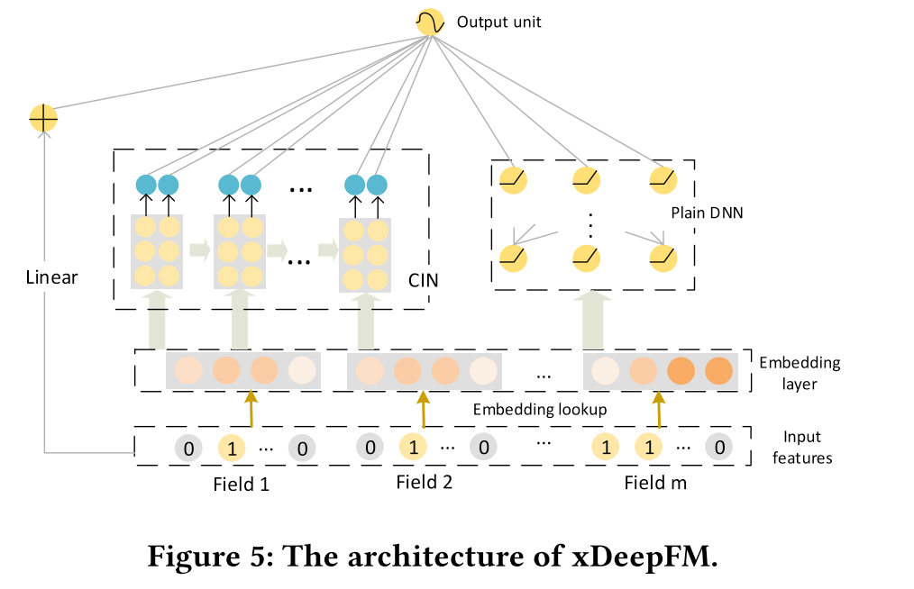
We can see from the below image that the architecture of xDeepFM is quite similar to DeepFM (that’s why they named it xDeepFM):
there are 3 parts, a linear module, a CIN module, and a DNN module
besides the CIN module, the rest 2 are the same as DeepFM
Compressed Interaction Network (CIN)
The CIN module is much more complicated than the Cross Network in DCN and FM in DeepFM. Let’s divide and explain it one by one.
A little bit of Math
To better understand the underline mechanism of CIN. Let’s recall some basic math.
To be simple, I will use 2x2 matrices for example. The same rules apply to any size matrix.
Suppose we have 2 matrices A and B:
Then the outer product is shown below, which can be thought of as multiplying B by every element of A. (This actually contains every possible combination for all the elements from A and B)
And the Hadamard product is an element-wise multiplication:
Outer product
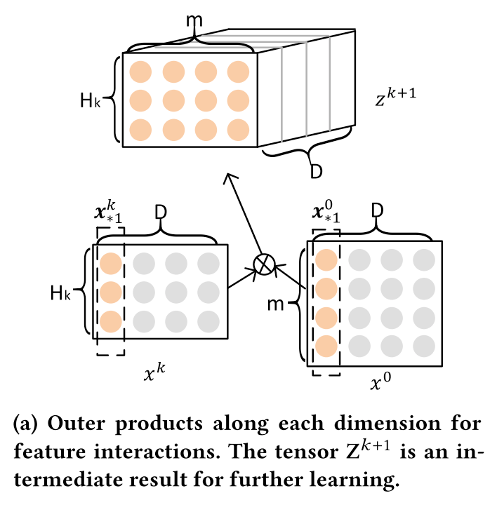
The first step is using an outer product to generate all the possible feature interactions.
Suppose the feature of the k-th layer has Hk fields and the dimension is D. And the input feature of the first layer X0 has m fields
Along the D dimension, generate the outer product one column by one column. This will generate a Hk*m dimension 2D tensor
Then slide along the D dimension, this will finally generate a Hk*m*D dimension 3D tensor
Notice that, the outer product is on a vector-wise level, there are no bit-wise interactions within each feature vector
CNN
The second step is using multiple feature maps from CNN to build a weighted sum of all the feature interactions
Apply multiple feature maps to the Hk*m tensor which represents all the feature interactions
Slide the feature maps along the D dimension. Suppose we have Hk+1 feature maps, then the output will be a (Hk+1)*D tensor

To be more formal, suppose in the k-th layer we have Hk feature maps and we use X to represent the feature vector (I simplify the formulas in the paper for easy understanding), then:
Here 1<=h<=Hk and X is a row vector in the picture, so the left X is an output row vector for the Hk layer.
How to understand this?
W is the weight of feature maps, so this formula is a combination of steps 1 and 2
Why in the picture, they are using an outer product, but in this formula there is only Hadamard products?
If we look closely, the right side of the formula is built for each row vector other than column-wise outer products in the step 1 picture. And it also contains all the combinations of feature interactions. Let’s split the A and B matrices into multiple row vectors:
\(\begin{align*} &W_{0,0}(A_0 \circ B_0) + W_{0,1}(A_0 \circ B_1) + W_{1,0}(A_1 \circ B_0) + W_{1,1}(A_1 \circ B_1) \\&= W_{0,0} \begin{bmatrix} a_{0,0} b_{0,0}, a_{0,1} b_{0, 1} \end{bmatrix} + W_{0, 1}\begin{bmatrix} a_{0,0} b_{1,0}, a_{0,1} b_{1, 1}\\ \end{bmatrix} \\&+ W_{1,0} \begin{bmatrix} a_{1,0} b_{0,0}, a_{1,1} b_{0, 1} \end{bmatrix} + W_{1,1} \begin{bmatrix} a_{1,0} b_{1,0}, a_{1,1} b_{1, 1}\\ \end{bmatrix} \end{align*}\)Then apply the weight to each feature interaction and finally sum all of them
The result is identical to the outer product + CNN process
Sum pooling
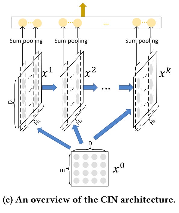
The last step is a sum-pooling operation.
For each layer, the sum-pooling operation is applied to the output features
The output features are also fed into the next layer, similar to an RNN
Then all the pooled features are concatenated to a flat tensor
Finally, a single dense layer is applied to the tensor and a weighted sum is calculated to get the logits
Time complexity
The cost of computing tensor Zk+1 (as shown in step 1) is O(mDH) time. Because we have H feature maps in one hidden layer, computing a T-layers CIN takes O(mDTH^2) time.
A T-layers plain DNN, by contrast, takes O(mDH+TH^2 ) time.
So the CIN is much slower than a plain DNN.
Show me the code
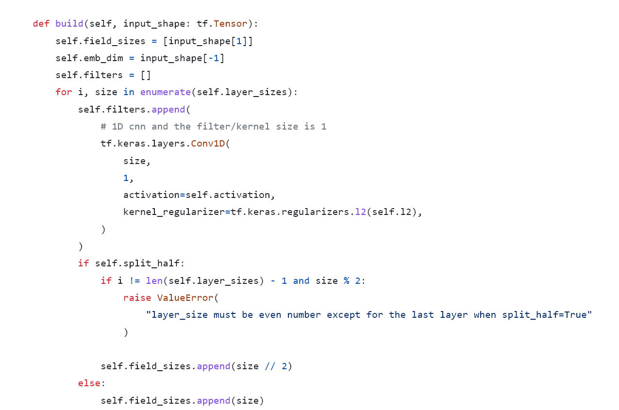
First, we need to store the field_sizes (the number of feature fields Hk) for each layer and initialize multiple 1D-CNNs based on the layer_size (filter maps).
The filter map size for the CNN is only 1. And the channels are actually the Hk*m 2D tensor in step 1
Then the filter map will slide along the D-dimensions
By default, the activation function for the CNN is linear, which shows the best performance in the paper
Notice that there is a split_half optimization parameter. If it’s true, the output of each CIN layer will be split into 2 pieces, one for the final output, and the other for the hidden input for the next layer.
We can refer to the original implementation from the paper author and DeepCTR. But their implementation leverages tf.split and tf.nn.conv1d to generate the outer product which is quite trivial and hard to understand. I simplified their code and use the tf.einsum and tf.keras.layers.Conv1D to construct the outer product easily. I also put the tensor shapes in the comment. The implementation is here:

Training
Let’s test this model on the MovieLens-1M dataset. All the 3 models use the same input features and the same CNN layer_sizes settings (100, 100, 100). And the rest hyperparameters are the same. Here quick means using split_half.
The quick version actually has better performance and training speed. Around 20% training speed improvement in my experiments
The Relu activation version for CNN is worse than the linear activation version. This is consistent with the paper’s result

Weekly Digest
Dealing with Train-serve Skew in Real-time ML Models: A Short Guide. A very detailed guide on how to solve data skew issues. A quick takeaway is using a feature store :)
PostgreSQL as a Vector Database: Create, Store, and Query OpenAI Embeddings With pgvector. Vector databases are super hot topics nowadays. Here is a tutorial of using a vector database in PostgreSQL
Mechanical Watch. How mechanical watch works? This dynamic illustration is so cool
One Life Isn’t Enough for All This Reading. “What we know is a drop, what we don’t know is an ocean.”
https://arxiv.org/pdf/1803.05170.pdf