Optimization in Multi Task Learning III

Gradient Surgery, Impartial Learning, Random Loss Weighting and Scalarization.

Long time no see all my friends.

Today, I’m wrapping up my final post on MTL (Multi-Task Learning) optimizers. There are several popular approaches I’d like to discuss. Ironically, by the end of 2023, two groundbreaking papers revealed that most previous methods are unreliable and largely ineffective. In the end, scalarization—a simple weighted sum of losses—is all we truly need. For context, feel free to revisit my earlier post.

Optimization in Multi Task Learning II

Gradient Surgery

Gradient surgery, or PCGrad (Project Conflicting Gradients)¹, is a multi-task optimization method designed to address conflicting gradients by projecting a task’s gradient onto the normal plane of another task’s gradient whenever a conflict is detected. The paper presenting PCGrad is well-structured, with its major contributions consisting of two key parts.

Previous studies primarily focused on the detrimental effects of gradient conflicts and proposed solutions but failed to clearly define what constitutes a gradient conflict or how to identify it. In contrast, PCGrad introduces three conditions of the multi-task optimization landscape that lead to detrimental gradient interference:

1. Different Gradient Directions: Gradients have a negative cosine similarity, indicating conflicting directions (a precondition for conflict).

2. Large Difference in Gradient Magnitude: Optimization becomes dominated by one task.

3. High Positive Curvature: Causes overestimation of the dominating task, leading to instability.

Let’s closely examine the illustrative example provided to better understand these concepts:

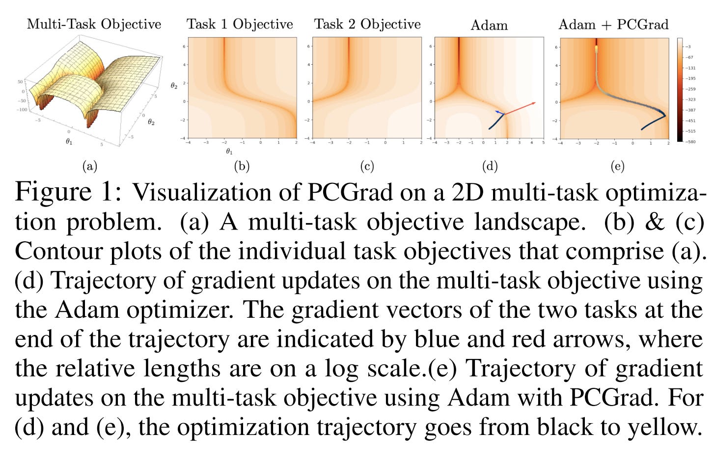
Many existing articles online fail to clearly explain this figure, so here’s a step-by-step breakdown:

1. Two Tasks and Parameters:
   The figure represents two tasks, with parameters θ1​ and θ2​.

2. Contour Plots (b) and (c):
   These show the loss changes corresponding to variations in θ. Both tasks exhibit high-curvature shapes, with task 2 having a higher curvature.

3. Gradient Interpretation:
   In contour plots, darker areas indicate smaller losses, so the optimization direction moves from lower to higher contours (bottom to top).

4. Picture (d):
   The small blue arrow on the left represents the gradient of task 2, while the large red arrow on the right represents task 1. Gradients are tangent to the loss curve. Here, the gradients conflict because they have a negative cosine similarity and significantly different magnitudes.

5. Picture (e):
   After applying PCGrad, the figure shows a smooth optimization trajectory, resolving the conflict.

The concept of high curvature can be challenging to grasp. Upon deeper research, it becomes clear that high positive curvature indicates a rapid change in gradient values. Regions with high curvature often have large gradient magnitudes, which can lead to overestimation. With a large gradient, even a moderately sized learning rate can cause updates that overshoot the optimal point.

From the example, it’s evident that large gradient values occur on both sides of the curve, further complicating optimization without techniques like PCGrad.

Projecting Conflict Gradients

The PCGrad method provides a simple yet effective solution to the problem of conflicting gradients in multi-task learning. If the gradients between two tasks are in conflict (i.e., their cosine similarity is negative), the procedure involves projecting the gradient of each task onto the normal plane of the gradient of the other task. This resolves conflicts by ensuring that the resulting gradients align with both tasks.

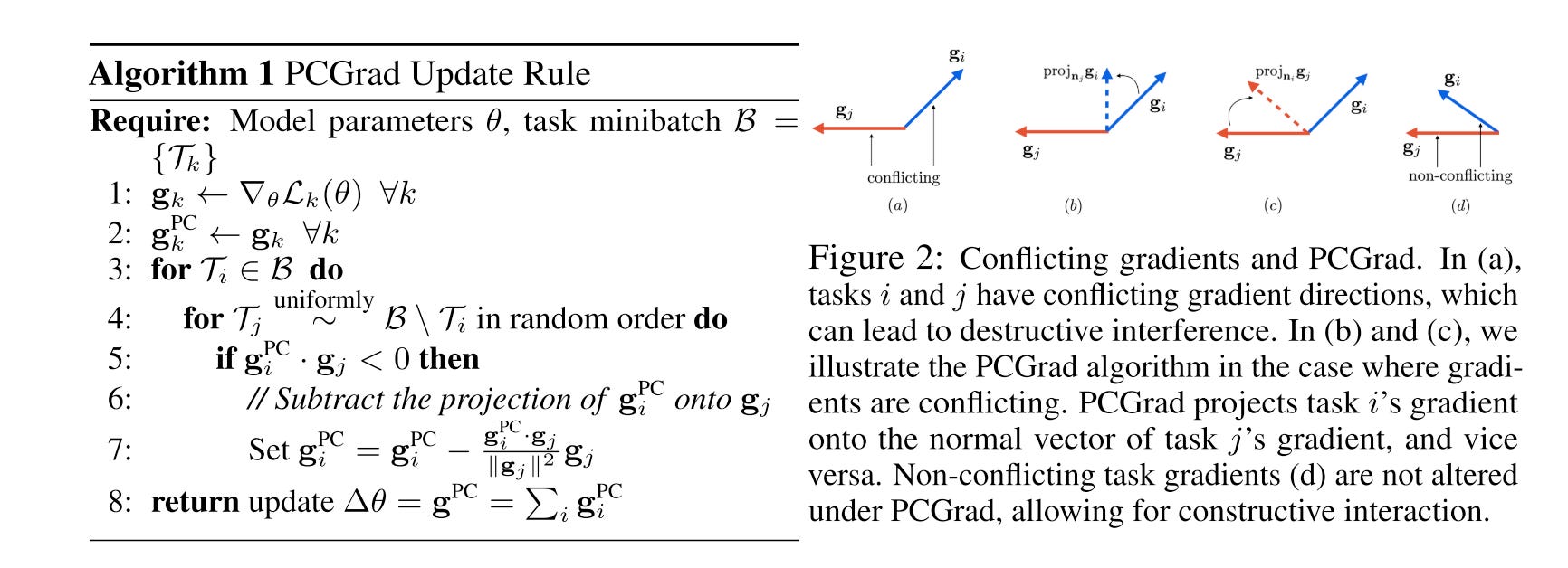
In Picture 2, tasks i and j initially have conflicting gradients. After projecting each gradient onto the normal plane of the other, the resulting gradients are non-conflicting, enabling smoother optimization.

The step-by-step algorithm is outlined below:

1. Calculate Gradients: Compute the gradient for each task.

2. Copy to PC Gradients: Duplicate the gradients to a separate PC gradient storage.

3. Conflict Check: For each task, randomly select another task and compute their cosine similarity.

4. Projection: If the gradients are conflicting (negative cosine similarity), project and update the PC gradient for the current task.

5. Gradient Descent: Sum all projected gradients and apply gradient descent

You might wonder whether modifying gradient directions and magnitudes would still allow the loss to converge. The paper addresses this concern both theoretically and experimentally. It demonstrates that applying PCGrad updates in a two-task setting with a convex and Lipschitz multi-task loss function L ensures convergence to the minimizer of L. Furthermore, PCGrad achieves a lower loss value after a single gradient update compared to standard gradient descent in multi-task learning.

This shows that the PCGrad method not only resolves gradient conflicts but also improves optimization efficiency and convergence performance.

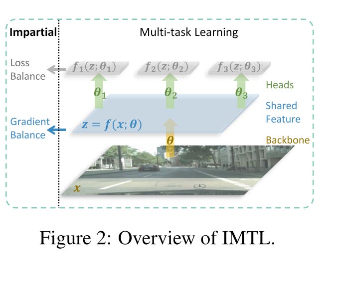
Impartial Multi-task Learning

IMTL² (impartial multi-task learning) , as the name suggests, aims to learn all tasks impartially. Specifically, for task-shared parameters, IMTL optimizes the scaling factors using a closed-form solution, ensuring that the aggregated gradient has equal projections onto each task. For task-specific parameters, it dynamically adjusts the task loss weights so that all losses remain at a comparable scale.

Another significant advantage of IMTL is its ability to be trained end-to-end without requiring heuristic hyper-parameter tuning. Additionally, it is versatile and can be applied to any type of loss function without assuming a specific distribution. This makes it much easier to use compared to methods like GradNorm or Uncertainty Weighting.

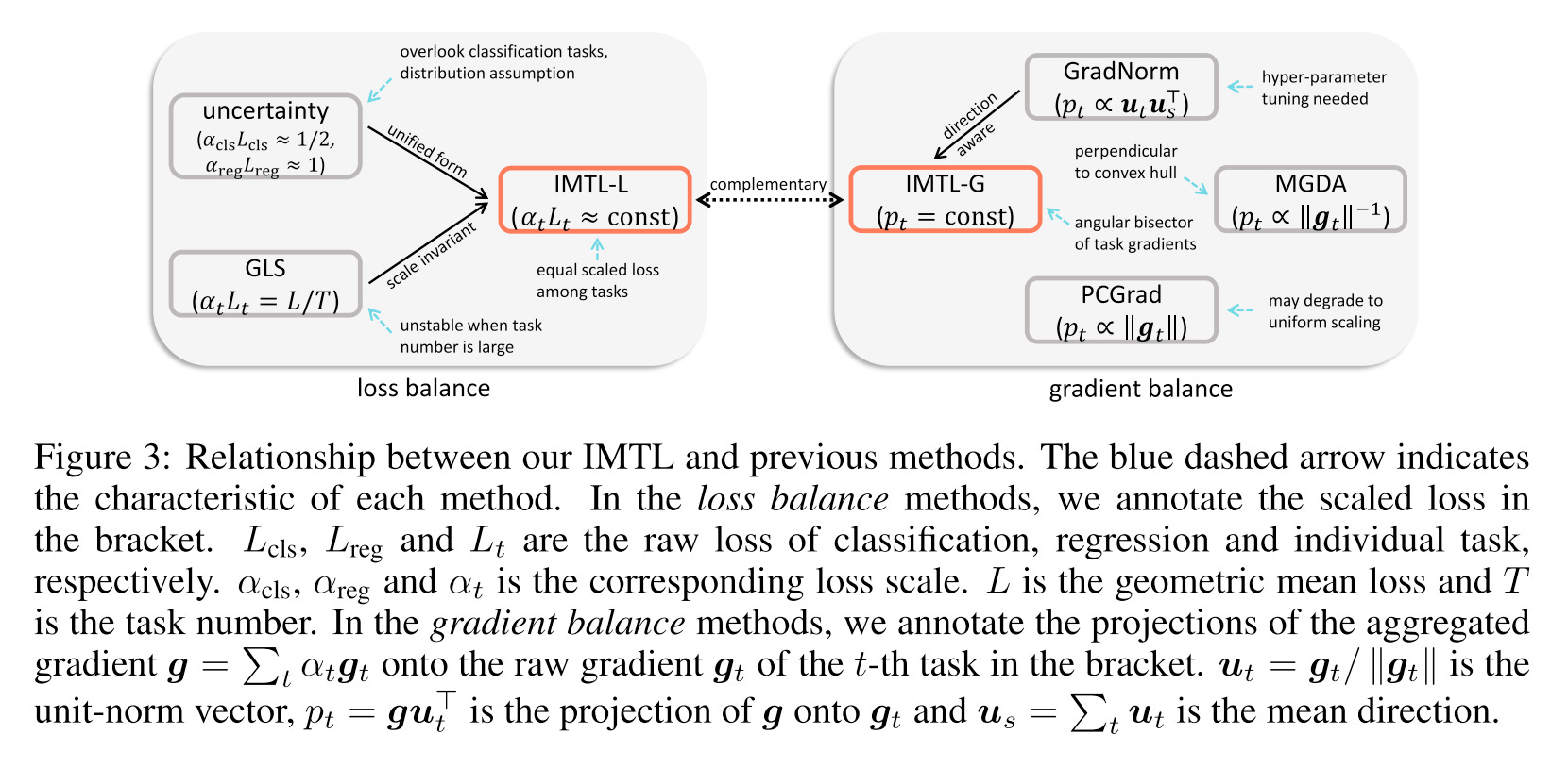
Existing multi-task optimization methods can be broadly classified into two categories: those that aim to achieve gradient balance and those that focus on loss balance. Gradient balance ensures even learning of task-shared parameters but overlooks task-specific ones. In contrast, loss balance prevents multi-task learning (MTL) from favoring tasks with larger loss scales but does not guarantee impartial learning of the shared parameters.

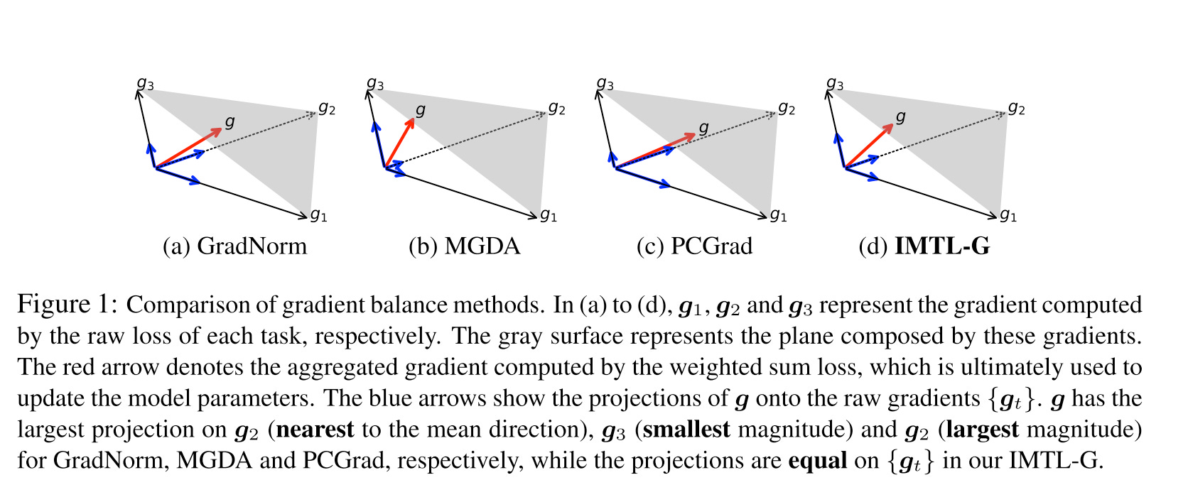
From the above picture, we can observe that for gradient balance, only IMTL-G (gradient) achieves equal projections onto each gradient direction.

For loss balance, the authors propose IMTL-L (loss), which automatically learns a loss-weighting parameter for each task. This ensures that the weighted losses have comparable scales, effectively canceling out the impact of differing loss scales across various tasks.

These two methods can also be combined to simultaneously balance both gradients and losses, providing a comprehensive solution for multi-task optimization.

Here is the detailed algorithm for the whole training process. Let’s dive into each process.

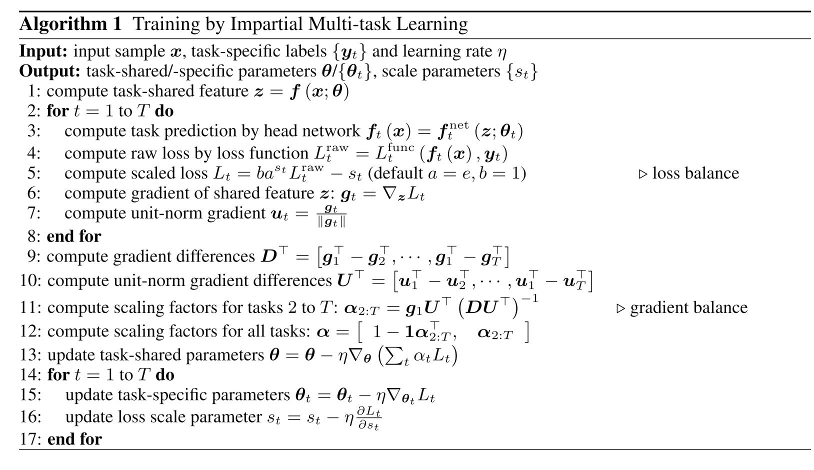
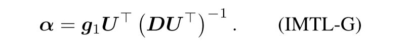
Gradient Balance: IMTL-G

The goal of IMTL-G is to treat all tasks equally so that they progress in the same speed and none is left behind. Formally, let u denote the norm vector of gradient g.

And they prove that this equation can be transformed to

Then the α is applied to scale the loss α*L, which is ultimately minimized by SGD to update the model. Notice that loop calculating the gradient for all the task is time consuming. Here the author borrow the idea from GradNorm and use the last shared feature Z as a surrogate of task-shared parameters.

Loss Balance: IMTL-L

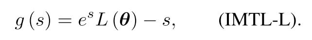
Loss balance is achieved by forcing the scaled losses α*L to be constant for all tasks, without loss of generality, the constant is 1. The simplest idea is to use the scaling factor as 1/L, but it’s sensitive to outliers and manifest severe oscillations. Then they introduce a mapping function h : R → R+ to transform the arbitrarily-ranged learnable scale parameters s to positive scaling factors h(s).

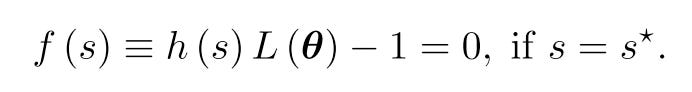
Assume the scaled loss g(s) is a differentiable convex function with respect to s, then its minimum is achieved if and only if s = s*, where the derivative of g(s) is zero:

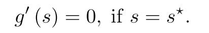
Since f(s) and g’(s) are both zero when s = s*. Then we can regard f(s) as the derivative of g(s):

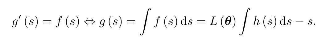
Notice that both ∫ h(s) and h(s) denotes loss scales, so that ∫ h(s) = Ch(s), here C is a constant. Then h(s) must be a exponential function. Take e as the Base, we will have.

Comparison

Compare to the previous methods, the IMTL have the following unique advantages:

1. No distribution assumption vs. Uncertainty Weighting

2. No hyper-parameter tuning vs. GradNorm

3. No clear discussion vs. PCGrad

4. MGDA focuses on small gradient magnitude tasks, break the task balance

For the experiment part, of course it shows it has better performance than any other optimizer. But here is the question, Is it truly reasonable to enforce all gradients to be impartial? If so, why?

The paper also leaves several questions unanswered.

Random Loss Weighting

Random Loss Weighting (RLW)³ is a straightforward yet effective approach. It involves sampling loss weights from a distribution, normalizing them, and then minimizing the aggregated loss using these normalized random weights. The paper demonstrates that training an MTL model with random weights sampled from a distribution can achieve performance comparable to state-of-the-art baselines. Additionally, RLW has a higher likelihood of escaping local minima compared to fixed loss weights.

The algorithm is simple and can be summarized as follows:

1. In each iteration, sample λ from a distribution p(λ), where p(λ) can be any distribution.

2. Normalize λ using an appropriate normalization function f.

3. Minimize the aggregated loss weighted by the normalized λ.

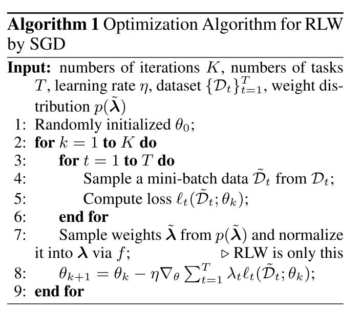
That’s all of the algorithm itself. Then they further theoretically prove that:

1. RLW method with the fixed step size has a linear convergence up to a radius around the optimal solution. It may requires more iterations to reach the same accuracy as FW ( fixed loss weights methods optimizing via SGD). But the experiments show that the impact is limited.

2. The extra randomness in the RLW method can help RLW to better escape sharp local minima and achieve a better generalization performance than FW

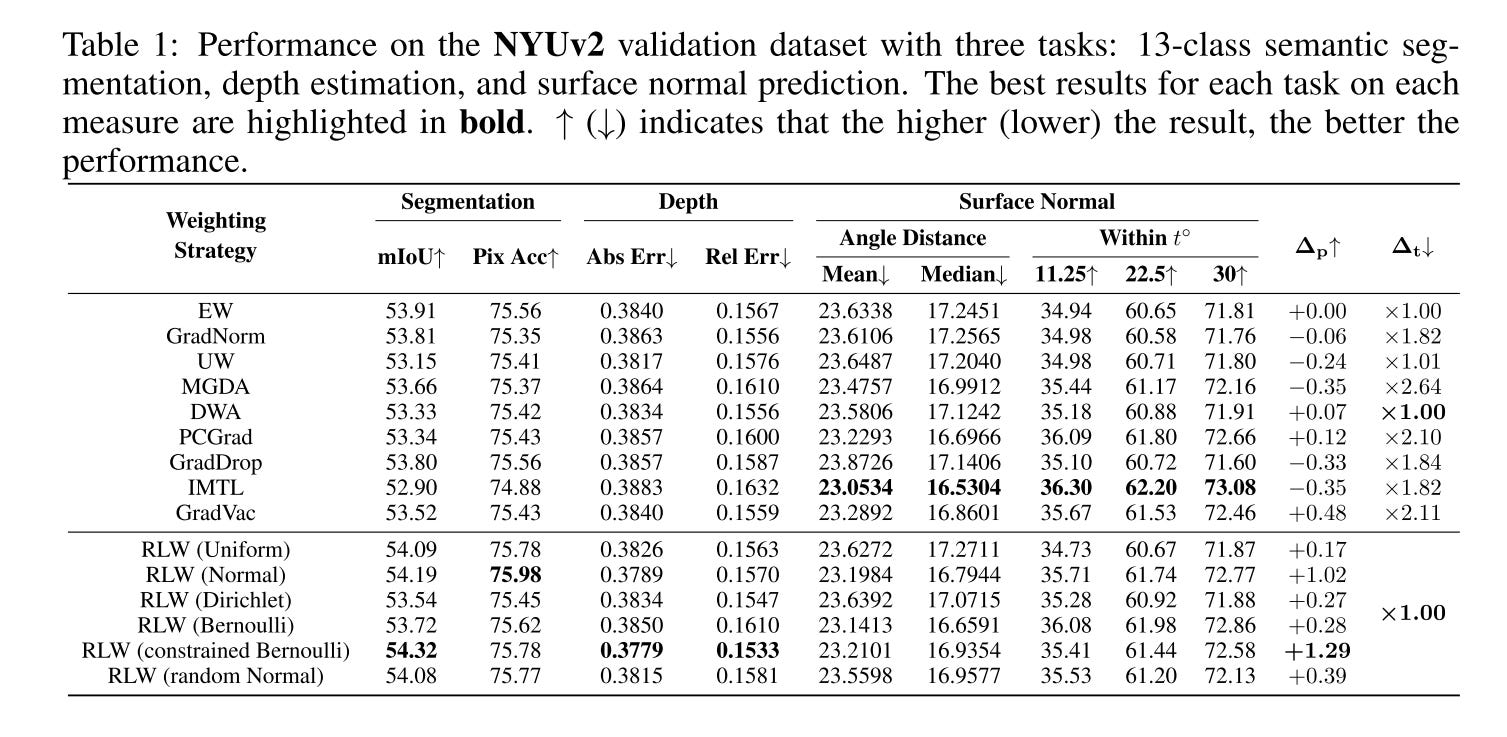
Experiment Result

From all the experiments result below, we can see that although RLW is not always the best, but it’s can achieve comparable performance vs. other popular optimizers.

Meanwhile, no single optimizer can outperform all the others.

This result brings us an important question:

Do Current Multi-Task Optimization Methods in Deep Learning Even Help?

This is the real paper title. And the conclusion in this paper is:

Despite the added design and computational complexity of these algorithms, MTO methods do not yield any performance improvements beyond what is achievable via traditional optimization approaches

1. The performance of multi-task models is sensitive to basic optimization parameters such as learning rate and weight-decay. Insufficient tuning of these hyper-parameters in the baselines, along with the complexity of evaluating multi-task models, can create a false perception of performance improvement

2. In some instances, the gains reported in the MTO literature are due to flaws in the experimental design. Often times these reported gains disappear with better tuning of the baseline hyperparameters. In addition, in a handful of cases, we were unable to reproduce the reported results

Background

Let’s first talk about some background to help us better understand the context.

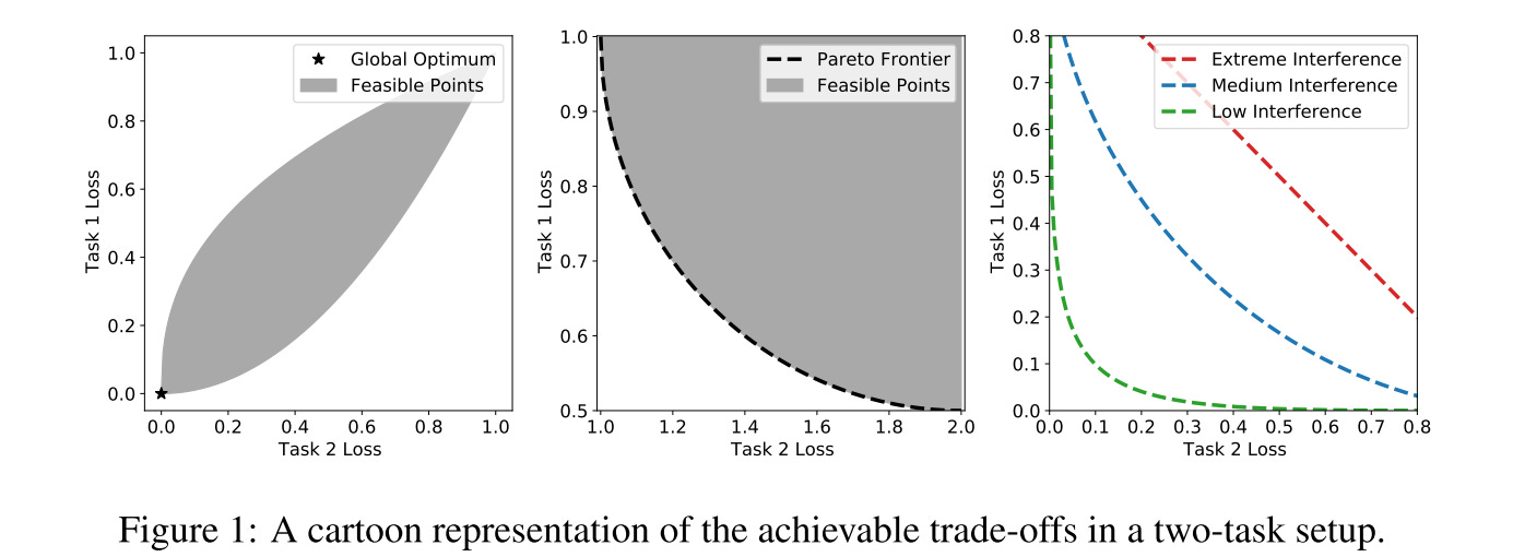
1. Figure 1 (left) provides a global optimum existing scenario example of MTL.

2. For most realistic setups, a globally optimal θ doesn’t exist. The middle picture provides a cartoon representation of the Pareto front for a two-task setup. The Pareto front represents the collection of parameters that achieve the best possible trade-off profile between the tasks.

3. Ideally, one would like to identify training protocols that push the trade-off curve towards the origin as much as possible, refer to Figure 1 (right).

The traditional approach for MTL optimization is scalarization, simply speaking, that is the weighted sum of all loss.

Here, w is a fixed vector of task weights determined by the practitioner beforehand. The algorithmic and computational simplicity of this approach has made scalarization highly popular in practice.

And in the convex setting it is provable that no algorithm can outperform properly chosen scalarization that has been trained to convergence.

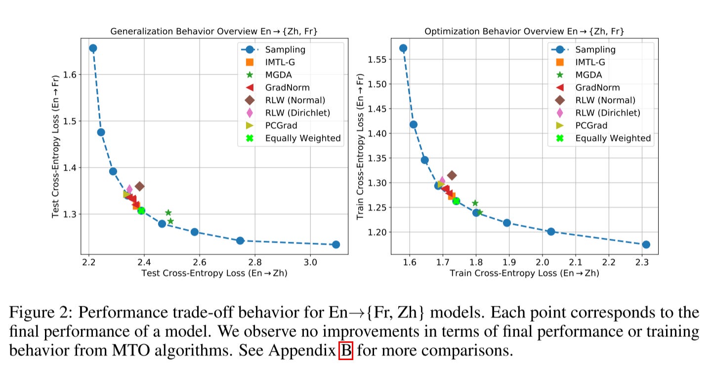
Experiments

They start the experiment by joint learning translation tasks. As we can see from this picture, no other MTL optimizer can outperform scalarization.

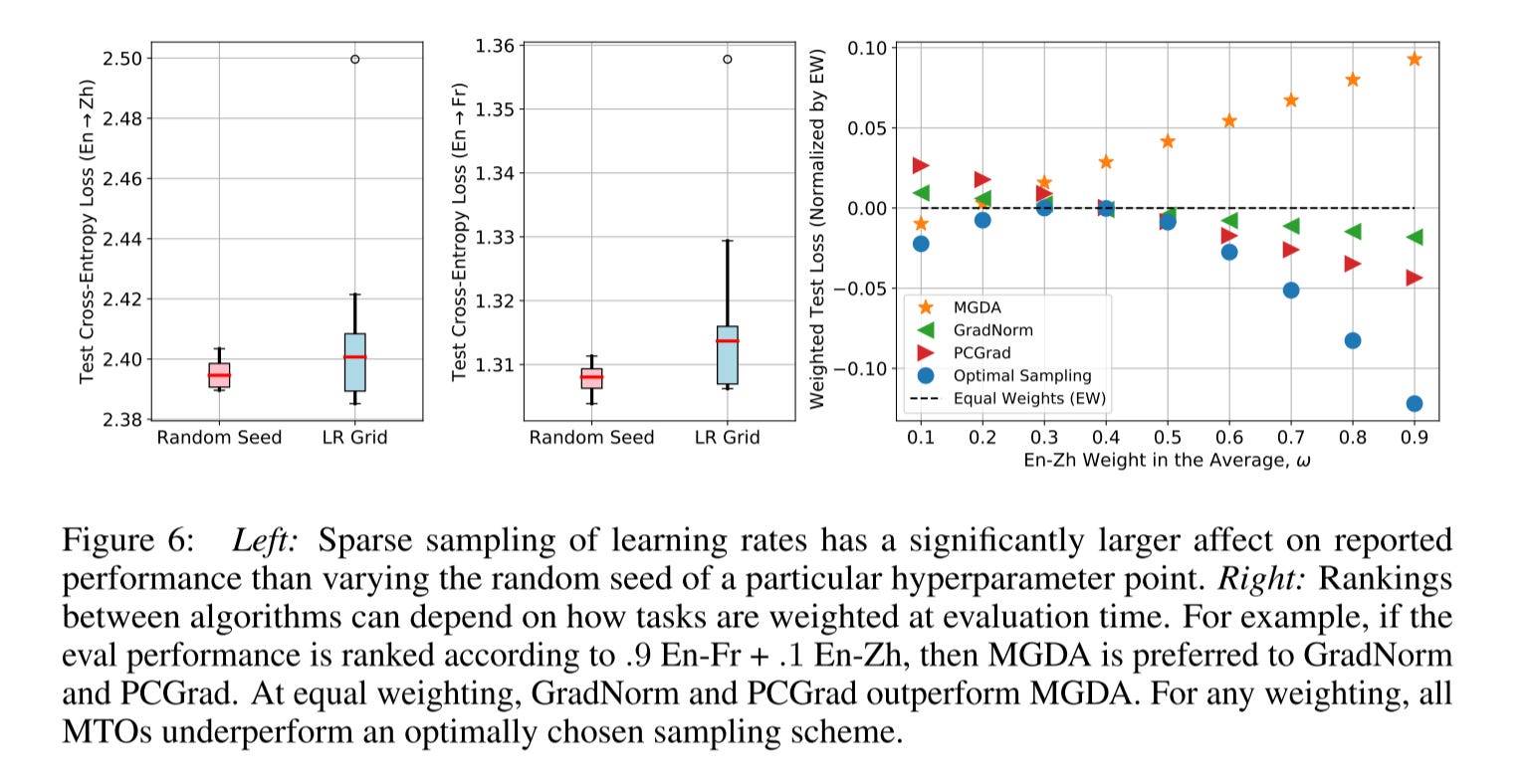
The model performances are highly sensitive to the choice of hyper-parameters. And estimating trial variance by rerunning multiple seeds is insufficient for concluding that performance gains from a new algorithm are significant when the hyperparameters are sampled on a sparse grid.

As we can see from the below picture, the learning rate selection has a much bigger impact than the optimizer itself.

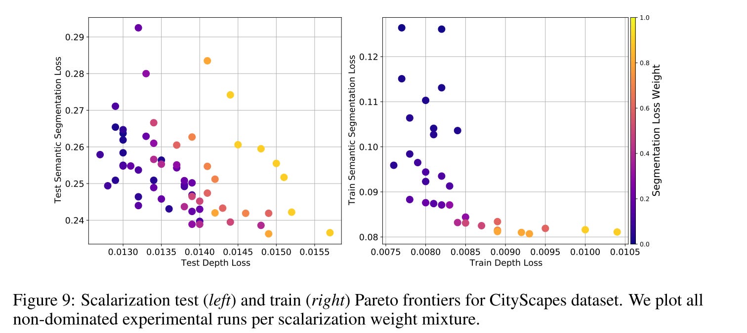
On the CityScapes experiment, loss balancing is still important. This dataset is popularly cast as a two-task problem with one task being 7-class semantic segmentation and the other being depth estimation. For CityScapes models, the segmentation task loss is an order of magnitude larger than the depth estimation task loss.

Appropriately balancing the different losses is crucial in achieving a desirable generalization behavior

The best result is achieved with segmentation task weight less than 0.2.

Here is another picture shows that hyper-parameter tuning is much more significant than the MTL optimizer itself. And the performance of MTL optimizers is highly dependent on the learning rate.

In conclusion, this paper directly argues that many of the previous experimental results in multi-task optimization are illusory, primarily due to improper hyperparameter tuning. The paper suggests that when hyperparameters are properly tuned, the performance improvements often attributed to MTO methods disappear, revealing that the gains were not genuinely due to the multi-task optimization techniques themselves.

In Defense of the Unitary Scalarization for Deep Multi-Task Learning

This paper⁴ argues that unitary scalarization where training simply minimizes the sum of the task losses without weighting is all we need. Unitary scalarization, coupled with standard regularization and stabilization techniques from single-task learning, matches or improves upon the performance of complex multi-task optimizers in popular supervised and reinforcement learning settings.

Let’s go straight to the experiments result.

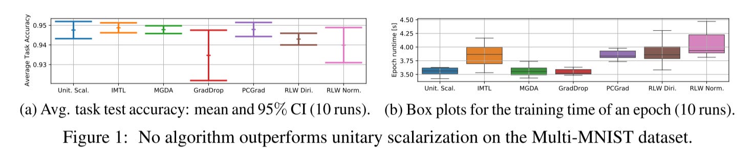
Similar to the previous paper, this one shows that no other optimizers outperform unitary scalarization.

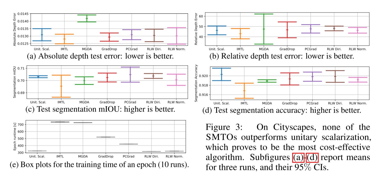
For the CityScrapes dataset, the authors found that unitary scalarization serves as a strong baseline. It's important to note that the loss is highly imbalanced between the two tasks. The previous paper emphasized the significance of loss balance, which contradicts the findings here. After double-checking the experimental setup, I noticed that the authors only conducted limited hyperparameter tuning for this dataset. Therefore, I still believe that loss balance is crucial, and I consider the results in this paper to be less reliable than those in the previous one.

Meanwhile, they point out that many papers report validation results, which can easily lead to overfitting and create the illusion of good performance.

What should we do for MTL tasks?

By the end of 2023, these are the latest developments in MTL tasks. It’s quite interesting to see how some paper results contradict others.

In summary, after reviewing all the experimental results and discussions, I would choose to first use IMTL-L to balance the loss, and then apply RLW to generate different loss weight combinations to explore the best result for all MTL tasks.

I don’t time to go over the papers in 2024 yet, if there is any other progress, I’m happy to know and share with you.

1. https://arxiv.org/pdf/2001.06782

2. https://openreview.net/forum?id=IMPnRXEWpvr

3. https://openreview.net/forum?id=OdnNBNIdFul

4. https://arxiv.org/pdf/2201.04122